2.4: Analog Modulation

The waveforms and spectra of the signals with common analog modulation methods are shown in Figure \(\PageIndex{1}\). The modulating signal is generally referred to as the baseband signal and it contains all of the information to be transmitted and interpreted at the receiver. The waveforms in Figure \(\PageIndex{1}\) are stylized. They are presented this way so that the effects of modulation can be more easily seen. The baseband signal (Figure \(\PageIndex{1}\)(a)) is shown as having a period that is not much greater than the period of the carrier (Figure \(\PageIndex{1}\)(b)). In reality there would be hundreds or thousands of RF cycles for each cycle of the baseband signal so that the highest frequency component of the baseband signal is a tiny fraction of the carrier frequency. In this situation the spectra shown on the right in Figure \(\PageIndex{1}\)(c–e) would be too narrow to enable any detail to be seen.

2.4.1 Amplitude Modulation

Amplitude Modulation (AM) is the simplest analog modulation method to implement. Here a signal is used to slowly vary the amplitude of the carrier according to the level of the modulating signal. With AM (Figure \(\PageIndex{1}\)(c)) the amplitude of the carrier is modulated, and this results in a broadening of the spectrum of the carrier, as shown in Figure \(\PageIndex{1}\)(c)(ii). This spectrum contains the original carrier component and upper and lower sidebands, designated as U and L, respectively. In AM, the two sidebands contain identical information, so all the information contained in the baseband signal is conveyed if just one sideband is transmitted.

The basic AM signal \(x(t)\) has the form

\[\label{eq:1}x(t)=A_{c}\left[1+my(t)\right]\cos (2\pi f_{c}t) \]

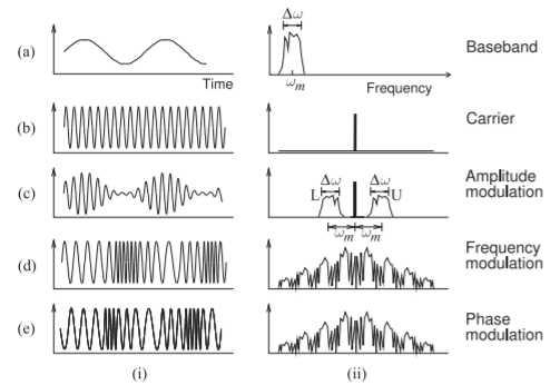
Figure \(\PageIndex{1}\): Basic analog modulation showing the (i) waveform and (ii) spectrum for (a) baseband signal; (b) carrier; (c) carrier modulated using amplitude modulation; (d) carrier modulated using frequency modulation; and (e) carrier modulated using phase modulation.

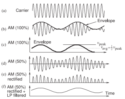
Figure \(\PageIndex{2}\): AM showing the relationship between the carrier and modulation envelope: (a) carrier; (b) \(100\%\) amplitude modulated carrier; (c) modulating or baseband signal; (d) \(50\%\) amplitude-modulated carrier; (e) rectified \(50\%\) AM modulated signal; and (f) rectified and lowpass (LP) filtered \(50\%\) modulated signal. The envelope contains only amplitude information and for AM the envelope is the same as the baseband signal.

where \(m\) is the modulation index, \(y(t)\) is the baseband information-bearing signal that has frequency components that are much lower than the carrier frequency \(f_{c}\), and the maximum value of \(|y(t)|\) is one. Provided that \(y(t)\) varies slowly relative to the carrier, \(x(t)\) looks like a carrier whose amplitude varies slowly. To get an idea of how slowly the amplitude varies in an actual system, consider an AM radio that broadcasts at \(1\text{ MHz}\) (which is in the middle of the AM broadcast band). The highest frequency component of the modulating signal corresponding to voice is about \(4\text{ kHz}\). Thus the amplitude of the carrier takes \(250\) carrier cycles to go through a complete amplitude variation. At all times a cycle of the modulated carrier, the pseudo-carrier, appears to be periodic, but in fact it is not quite.

The concept of the envelope of a modulated RF signal is introduced in Figure \(\PageIndex{2}\). The envelope is an important concept and is directly related to the distortion introduced by analog hardware and to the DC power requirements which determines the battery life for mobile radios. Figure \(\PageIndex{2}\)(a) is the carrier and the amplitude-modulated carrier is shown in Figure \(\PageIndex{2}\)(b). The outline of the modulated carrier is called the envelope, and for AM this is identical to the modulating, i.e. baseband, signal. The envelope is shown again in Figure \(\PageIndex{2}\)(c). At the peak of the envelope, the RF signal has maximum short-term power (considering the power of a single RF cycle). With \(100\%\) AM, \(m = 1\) in Equation \(\eqref{eq:1}\), there is no short-term RF power when the envelope is at its minimum. The modulated signal with \(50\%\) modulation, \(m = 0.5\), is shown in Figure \(\PageIndex{2}\)(d) and at all times there is an appreciable RF signal power.

Very simple analog hardware is required to demodulate the basic amplitude modulated signal, that is an AM signal with a carrier and both sidebands. The receiver requires bandpass filtering to select the channel from the incoming radio signal then rectifying the output of the bandpass filter. The waveform after rectification of a \(50\%\) AM signal is shown in Figure \(\PageIndex{2}\)(e) and contains frequency components at baseband and sidebands around harmonics of the carrier, and the harmonics of the carrier itself. Lowpass filtering of the rectified waveform extracts the original baseband signal and completes demodulation, see Figure \(\PageIndex{2}\)(f). The only electronics required is a

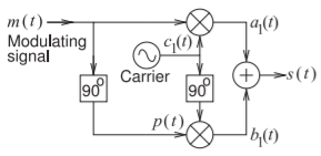
Figure \(\PageIndex{3}\): Hartley modulator implementing singlesideband suppressed-carrier (SSB-SC) modulation. The “\(90^{\circ}\)” blocks shift the phase of the signal by \(+90^{\circ}\). The mixer indicated by the circle with a cross is an ideal multiplier, e.g. \(a_{1}(t) = m(t) \cdot c_{1}(t)\).

single diode. The disadvantage is that more spectrum is used than required and the largest signal is the carrier that conveys no information but causes interference in other radios. Without the carrier and both sidebands being transmitted it is necessary to use DSP to demodulate the signal.

It is not possible to represent an actual baseband signal in a simple way and undertake the analytic derivations that illustrate the characteristics of modulation. Instead it is usual to use either a one-tone or two-tone signal, derive results, and then extrapolate the results for a finite bandwidth baseband signal. For a single-tone baseband signal \(y(t) = \cos (\omega_{m}t + \phi )\), then the basic AM modulated signal, from Equation \(\eqref{eq:1}\), is

\[\begin{align}x(t)&=\left[1+m\cos (\omega_{m}t+\phi )\right]\cos (\omega_{c}t)\nonumber \\ \label{eq:2}&=\cos (\omega_{c}t)+\frac{1}{2}m\left[\cos ((\omega_{c}-\omega_{m})t-\phi)+\cos ((\omega_{c}+\omega_{m})t+\phi )\right]\end{align} \]

which has three (radian) frequency components, one at the carrier frequency \(\omega_{c}\), one just below the carrier at \(\omega_{c}-\omega_{m}\), and one just above at \(\omega_{c} +\omega_{M}\) (since \(\omega_{m} ≪ \omega_{c}\)). The extension to a finite bandwidth baseband signal, see Figure \(\PageIndex{1}\)(a)(ii), is to imagine that ωm ranges from a lower value \(\omega_{m}− \frac{1}{2}\Delta\omega\) to a higher value \(\omega_{m}+ \frac{1}{2}\Delta\omega\). The discrete tones in the modulated signal below and above the carrier then become finite bandwidth sidebands with a lower sideband L centered at \(\omega_{c} −\omega_{m}\) and an upper sideband U centered at at \((\omega_{c} +\omega_{m})\) each having the same bandwidth, \(\Delta\omega\), as the baseband signal, see Figure \(\PageIndex{1}\)(c)(ii).

The AM modulator described so far produces a modulated signal with a carrier and two sidebands. This modulation is called double-sideband (DSB) modulation. There is identical information in each of the sidebands and so only one of the sidebands needs to be transmitted. The carrier contains no information so if only one sideband was transmitted then the received single-sideband (SSB) suppressed-carrier SC (together SSB-SC) signal has all of the information needed to recover the original baseband signal. However the simple demodulation process using rectification as described earlier in this section no longer works. The receiver needs to use DSP but the spectrum is used efficiently.

One circuit that implements SSB-SC AM is the Hartley modulator shown in Figure \(\PageIndex{3}\). As will be seen, this basic architecture is significant and used in all modern radios. In modern radios the Hartley modulator, or a variant, takes a modulated signal which is centered at an intermediate frequency and shifts it up in frequency so that it is centered at another frequency a little below or a little above the carrier of the Hartley modulator.

In a Hartley modulator both the modulating signal \(m(t)\) and the carrier are multiplied together in a mixer and then also \(90^{\circ}\) phase-shifted versions are mixed before being added together. The signal flow is as follows beginning with \(m(t) = \cos (\omega_{m}t +\phi),\: p(t) = \cos (\omega_{m}t + \phi − π/2) = \sin (\omega_{m}t + \phi)\) and carrier signal \(c_{1}(t)=\cos(\omega_{c}t)\):

\[\begin{align}a_{1}(t)&=\cos (\omega_{m}t+\phi )\cos (\omega_{c}t)=\frac{1}{2}\left[\cos ((\omega_{c}-\omega_{m})t-\phi )+\cos ((\omega_{c}+\omega_{m})t+\phi )\right]\nonumber \\ b_{1}(t)&=\sin (\omega_{m}t+\phi )\sin (\omega_{c}t)=\frac{1}{2}\left[\cos ((\omega_{c}-\omega_{m})t-\phi )-\cos ((\omega_{c}+\omega_{m})t+\phi )\right]\nonumber \\ \label{eq:3} s(t)&=a_{1}(t)+b_{1}(t)=\cos ((\omega_{c}-\omega_{m})t-\phi )\end{align} \]

and so the lower sideband (LSB) is selected. An interesting observation is that the phase, \(\phi\), of the baseband signal is also translated up in frequency. A feature that is not exploited in AM but is in digital modulation.

2.4.2 Phase Modulation

In phase modulation (PM) the phase of the carrier depends on the instantaneous level of the baseband signal. The phase-modulated carrier is shown in Figure \(\PageIndex{1}\)(e)(i) and it looks like the frequency of the modulated carrier is changing. What is actually happening is that when the phase is changing most quickly the apparent frequency of the RF waveform changes. Here, as the baseband signal is decreasing, the phase shift reduces and the effect is to increase the apparent frequency of the RF signal. As the baseband signal increases, the effect is to reduce the apparent frequency of the modulated RF signal. The result is that with PM is that the bandwidth of the time-varying signal is spread out, as seen in Figure \(\PageIndex{4}\). PM can be implemented using a phase-locked loop (PLL) but further details will be skipped here.

Consider a phase-modulated signal \(s(t) = \cos(\omega_{c}t+\phi (t))\) where \(\phi (t)\) is the baseband signal containing the information to be transmitted. The spectrum of \(s(t)\) can be determined by simplifying \(\phi (t)\) as a sinusoid with frequency \(f_{m} = 2π\omega_{m}\) so that \(\phi (t) =\beta \cos(\omega_{m}t)\) where \(\beta\) is the phase modulation index. (The maximum possible phase change is \(±\pi\) and then \(\beta=\pi\).) The phase-modulated signal becomes

\[\begin{align}s(t)&=\cos (\omega_{c}t+\beta\cos(\omega_{m}t)])\nonumber \\ \label{eq:4}&=\cos(\omega_{c}t)\cos(\cos(\beta\omega_{m}t))-\sin(\omega_{c}t)\sin(\cos(\beta\omega_{m}t))\end{align} \]

which has the Bessel function-based expansion

\[\begin{align} &s(t)=J_{0}(\beta )\cos (\omega_{c}t) \nonumber \\ &+J_{1}(\beta )\cos (\omega_{c}+\omega_{m})t+\pi /2)+J_{1}(\beta)\cos (\omega_{c}-\omega_{m})t+\pi /2)\nonumber \\ &+J_{2}(\beta )\cos (\omega_{c}+2\omega_{m})t+\pi )+J_{2}(\beta )\cos (\omega_{c}-2\omega_{m})t+\pi ]\nonumber \\ \label{eq:5}&+J_{3}(\beta )\cos (\omega_{c}+3\omega_{m})t+3\pi /2)+J_{3}(\beta )\cos (\omega_{c}-3\omega_{m})t+3\pi /2)+\ldots\end{align} \]

where \(J_{n}\) is the Bessel function of the first kind of order \(n\). The spectrum of this signal is shown in Figure \(\PageIndex{4}\)(a) which consists of discrete tones grouped as lower- and upper-sideband sets centered on the carrier at \(f_{c}\). The discrete tones in the sidebands are separated from each other and from \(f_{c}\) by \(f_{m}\). The sidebands have lower amplitude further away from the carrier.

If the modulating signal has a finite bandwidth, approximated by \(f_{m}\) varying from a minimum value, \((f_{m} −\Delta f)\) up to the maximum frequency \((f_{m} +\Delta f)\), then the spectrum of the modulated signal becomes that shown in Figure \(\PageIndex{4}\)(b), with the centers of adjacent sidebands separated by \(f_{m}\) and the first sidebands separated from the carrier by fm as well. This is DSB

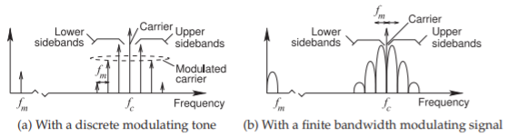
Figure \(\PageIndex{4}\): Spectrum of a phase-modulated carrier which includes the carrier at \(f_{c}\) and upper and lower sidebands with the spectrum of the discrete modulating signal at \(f_{m}\).

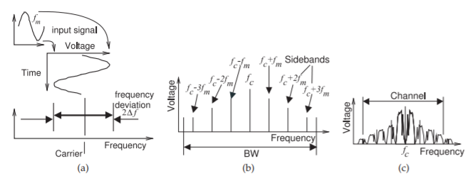
Figure \(\PageIndex{5}\): Frequency modulation: (a) sinusoidal baseband signal shown varying the frequency of the carrier and so FM modulating the carrier; (b) the spectrum of the resulting FM-modulated waveform; and (c) spectrum of the modulated carrier when it is modulated by a broadband baseband signal such as voice.

modulation and there is a carrier (so it is not suppressed). The sidebands do not carry identical information and several, perhaps three below and three above the carrier, are required to enable demodulation of a PM signal. Thus a rather large bandwidth is required to transmit the modulated signal.

2.4.3 Frequency Modulation

The other analog modulation schemes commonly used is frequency modulation (FM), see Figure \(\PageIndex{1}\)(d). The signals produced by FM and PM appear to be similar; the difference is in how the signals are generated. In FM, the amplitude of the baseband signal determines the frequency of the modulated carrier. Consider the FM waveform in Figure \(\PageIndex{1}\)(d)(i). When the baseband signal is at its peak value the modulated carrier is at its minimum frequency, and when the signal is at is lowest value the modulated carrier is at its maximum frequency. (Depending on the hardware implementation it could be the other way around.) The result is that the bandwidth of the time-varying signal is spread out, as seen in Figure \(\PageIndex{5}\).

One way of implementing the FM modulator is to use a voltage-controlled oscillator (VCO) with the baseband signal controlling the frequency of an oscillator. An FM receiver must compress, in frequency, the transmitted signal to re-create the original narrower bandwidth baseband signal. FM demodulation can be thought of as providing signal enhancement or equivalently noise suppression in a process that can be called analog processing gain. Only the components of the original FM signals are coherently collapsed to a narrower bandwidth baseband signal while noise, being uncorrelated, is still spread out (although rearranged). Thus the ratio of the signal to noise powers increases, as after demodulation only the power of the noise in the smaller bandwidth of the baseband signal is important. Thus compared to AM, FM significantly increases the tolerance to noise that may be added to the signal during transmission. PM has the same property, although the details of modulation and demodulation are different. For both FM and PM signals the peak amplitude of the RF phasor is equal to the average amplitude, and so the PMEPR is \(1\) or \(0\text{ dB}\).

Consider an FM signal \(s(t) = \cos([\omega_{c} + x(t)]t)\) where \(x(t)\) is the baseband signal containing the information to be transmitted. The spectrum of \(s(t)\) can be determined by simplifying \(x(t)\) as a sinusoid with frequency \(f_{m} = 2π\omega_{m}\) so that \(x(t) = \beta\cos(\omega_{m}t)\) where \(\beta\) is the frequency modulation index. The FM signal becomes

\[\begin{align}s(t)&=\cos([\omega_{c}+\beta\cos(\omega_{m}t)]t)\nonumber \\ \label{eq:6}&=\cos(\omega_{c}t)\cos(\cos(\omega_{m}t)\beta t)-\sin(\omega_{c}t)\sin(\cos(\omega_{m}t)\beta t)\end{align} \]

which has the Bessel function-based expansion

\[\begin{align}&s(t)=J_{0}(\beta t)\cos (\omega_{c}t)\nonumber \\&-J_{1}(\beta )\sin(\omega_{c}+\omega_{m})t+\pi /2)-J_{1}(\beta t)\sin(\omega_{c}-\omega_{m})t+\pi /2)\nonumber \\ &-J_{2}(\beta t)\cos(\omega_{c}-2\omega_{m})t+\pi )+K_{2}(\beta t)\cos (\omega_{c}-2\omega_{m})t+\pi ]\nonumber \\ \label{eq:7}&+J_{3}(\beta t)\sin(\omega_{c}+3\omega_{m})t+3\pi /2)+J_{3}(\beta t)\sin(\omega_{c}-3\omega_{m})t+3\pi /2)+\ldots\end{align} \]

where \(J_{n}\) is the Bessel function of the first kind of order \(n\). The spectrum of this signal is shown in Figure \(\PageIndex{5}\)(b) which consists of discrete tones grouped as lower- and upper-sideband sets centered on the carrier at \(f_{c}\). The discrete tones in the sidebands are separated from each other and from \(f_{c}\) by \(f_{m}\). The sidebands have lower amplitude further away from the carrier.

If the modulating signal has a finite bandwidth, approximated by \(f_{m} = \omega_{m}/(2π)\) varying from a minimum value (\(f_{m}− \Delta f)\) up to the maximum frequency \((f_{m}+\Delta f)\), then the spectrum of the modulated signal becomes that shown in Figure \(\PageIndex{5}\)(c) with the centers of adjacent sidebands separated by \(f_{m}\) and the first sidebands from the carrier by \(f_{m}\) as well. This is DSB modulation and there is a carrier (so it is not suppressed but is smaller than with AM). The sidebands do not carry identical information and several, perhaps three on either side of the carrier, are required to enable demodulation of an FM signal. Thus a rather large bandwidth to required to transmit the modulated signal as it is not sufficient to transmit just one sideband to enable demodulation.

Carson's Rule

Frequency- and phase-modulated signals have a very wide spectrum and the bandwidth required to reliably transmit a PM or FM signal is subjective. The best accepted criterion for determining the bandwidth requirement is called Carson’s bandwidth rule or just Carson’s rule [7, 8].

An FM signal is shown in Figure \(\PageIndex{5}\). In particular, Figure \(\PageIndex{5}\)(a) shows the FM function. The level (typically voltage) of the baseband signal determines the frequency deviation of the carrier from its unmodulated value. The frequency shift when the modulating signal is a DC value \(x_{m}\) at its maximum amplitude is called the peak frequency deviation, \(\Delta f\). So, if the modulating signal changes very slowly, the bandwidth of the modulated signal is \(2\Delta f\).

A rapidly varying sinusoidal modulating signal produces a modulated signal with many discrete sidebands as seen in Figure \(\PageIndex{5}\)(b). If the modulating baseband signal is broadband, then the sidebands have finite bandwidth as seen in Figure \(\PageIndex{5}\)(c) and many are required to recover the original baseband signal. These sidebands continue indefinitely in frequency but rapidly reduce in power away from the frequency of the unmodulated carrier. Carson’s rule provides an estimate of the bandwidth that contains \(98\%\) of the energy. If the maximum frequency of the modulating signal is \(f_{m}\), and the maximum value of the modulating waveform is \(x_{m}\) (which would produce a frequency deviation of \(\Delta f\) if it is DC), then Carson’s rule is that the

\[\label{eq:8}\text{bandwidth required }=2\times (f_{m}+\Delta f) \]

Narrowband and Wideband FM

The most common type of FM signal, as used in FM broadcast radio, is called wideband FM, as the maximum frequency deviation is much greater than the highest frequency of the modulating or baseband signal, that is, \(\Delta f ≫ f_{m}\). In narrowband FM, \(\Delta f\) is close to \(f_{m}\). Narrowband FM uses less bandwidth but requires a more sophisticated demodulation technique.

Example \(\PageIndex{1}\): PAPR and PMEPR of FM Signals

Consider FM signals close in frequency but whose spectra do not overlap.

1. What are PAPR and PMEPR of just one FM signal?
2. What are PAPR and PMEPR of a signal comprised of two uncorrelated narrowband FM signals each having a small fractional bandwidth and having the same average power.

Solution

1. An FM signal has a constant envelope just like a single sinusoid, and so \(\text{PAPR} = 1.414 = 3.01\text{ dB}\) and \(\text{PMEPR} = 1 = 0\text{ dB}\).
2. Since the modulation is relatively slow, each of the FM signals will look like single tone signals and the combined signal will look like a two-tone signal. However this is not enough to solve the problem. A thought experiment is required to determine the largest pseudo-carrier when the FM signals combine. If the amplitude of each tone is \(X\), then the amplitude when the FM signal waveforms align is \(2X\). (This is the same as the peak of a two-tone signal but arrived at differently.) Then
   \[P_{\text{avg}}=\text{sum of the powers of each FM signal }=2k\frac{1}{2}X^{2}\nonumber \]
   where \(k\) is a proportionality constant. For PAPR,
   \[\label{eq:9}P_{P}=k(2X)^{2}\quad\text{and}\quad\text{PMEPR}=\frac{P_{P}}{P_{\text{avg}}}=\frac{k(2X)^{2}}{2k\frac{1}{2}X^{2}}=4=6.0\text{ dB} \]
   For PMEPR, \(P_{\text{PEP}}=\text{ power of the pseudo-carrier }=k\frac{1}{2}(2X)^{2}\)
   and
   \[\label{eq:10}\text{PMEPR}=\frac{P_{P}''}{P_{\text{avg}}}=\frac{k\frac{1}{2}(2X)^{2}}{2k\frac{1}{2}X^{2}}=2=3.0\text{ dB} \]

2.4.4 Analog Modulation Summary

Analog modulation was used in the first radios and in 1G cellular radios. Radio transmission using analog modulation, i.e. analog radio, has almost ceased as it does not use spectrum efficiently. Digital modulation along with error correction, can pack much more information in a limited bandwidth. A final comparison of the analog modulation techniques is given in Figure 2.5.1 emphasizing the PMEPR of AM and FM. The PMEPR of PM is the same as for FM.

One particular event in the development of radio is illustrative of the relationship of technology and business interests. Frequency modulation was invented by Edwin H. Armstrong and patented in 1933 [9, 10]. FM is virtually static free and clearly superior to AM radio. However, it was not immediately adopted largely because AM radio was established in the 1930s, and the adoption of FM would have resulted in the scrapping of a large installed infrastructure (seen as a commercial catastrophe) and so the introduction of FM was delayed by decades. The best technology does not always win immediately! Commercial interests and the large investment in an alternative technology have a great deal to do with the success of a technology [11].

With FM and PM there are two sets of sidebands with one set above the carrier frequency and the other set below. The carrier itself is low-level but is not completely suppressed. Now SSB modulation refers to producing just one of the sideband sets. There is such as thing as SSB FM with just a few sidebands below (or above) the carrier but it is more like a combination of FM and AM [12], and was never deployed.