2.5: Digital Modulation

Digital radio transmits bits by creating discrete states, usually discrete amplitudes and phases of a carrier. The process of creating these discrete states from a digital bitstream is called digital modulation. A state is established at a particular time called a clock tick. What that means is that the

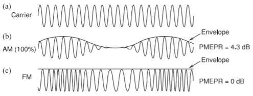
Figure \(\PageIndex{1}\): Comparison of \(100\%\) AM and FM highlighting the envelopes of both: (a) carrier; (b) AM signal; and (c) FM signal with constant envelope.

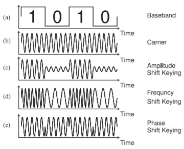
Figure \(\PageIndex{2}\): Modes of digital modulation: (a) modulating bitstream; (b) carrier; (c) carrier modulated using amplitude shift keying (ASK); (d) carrier modulated using frequency shift keying (FSK); and (e) carrier modulated using binary phase shift keying (BPSK).

information in the signal is the state of the waveform, such as the amplitude and the phase of a phasor, at every clock tick such as every microsecond. The time it takes to go from one state to another (a clock tick interval) defines the bandwidth of the modulated signal. For example, if a clock tick is at every microsecond the bandwidth of the modulated signal is about one megahertz as it takes about one microsecond to go from one state to another. The inverse relationship of the interval between clock ticks to bandwidth is only approximate (as will be seen when software-defined radio is considered in a future chapter).

One important digital modulation method does not fit with the description above. This is Frequency Shift Keying (FSK) modulation where the carrier is set to a particular frequency at each clock tick.

The basic digital modulation formats are shown in Figure \(\PageIndex{2}\). The fundamental characteristic of digital modulation is that there are discrete states, each of which is also known as a symbol, with a symbol defining the value of one or more bits. For example, the states are different frequencies in FSK and different phases in phase shift keying (PSK). With the modulated waveforms shown in Figure \(\PageIndex{2}\) there are only two states, which is the same as saying that there are two symbols, each symbol having one bit of information (either \(0\) or \(1\)). With multiple states groups of bits can be represented.

In this section many methods of digital modulation are described. The first few methods are binary modulation methods with just two symbols with one symbol indicating that a single bit is ‘\(0\)’ and the other symbol indicating that it is a ‘\(1\)’. Then four-state modulation is introduced with four symbols with each symbol indicating the values of two bits. Higher-order modulation schemes can send more than more bits per symbol and thus more bits per second (bits/s) per hertz of bandwidth. There is a limit to the number of symbols as the “distance” between symbols becomes smaller and the effect of noise, interference, and circuit distortion can cause a symbol to be misinterpreted as another. A modulation method that sends more bits per symbol is said to have higher modulation efficiency. This and other metrics that enable modulation methods to be compared are defined in the next subsection.

2.5.1 Modulation Efficiency

With digital modulation, the information being sent is in the form of bits and it is possible to send more that one bit per second in one hertz of bandwidth. This is because in digital modulation there can be several bits per symbol, however the bandwidth of the modulated signal is determined by the rate of change from one state to another, whereas the number of bits per transition depends on the number of states. It is important for the transition to be no faster than required so as to minimize bandwidth.

The ratio of the bit rate in bits per second (\(\text{bits/s}\)) to the bandwidth (BW) in hertz is called the modulation efficiency, \(\eta_{c}\), and has the units of bits per second per hertz (\(\text{bits/s/Hz}\)). The modulation efficiency is also called the channel efficiency, hence the subscript \(c\) on \(\eta_{c}\). The bits here are the gross bits which includes the information bits and bits added for error correction and others added to aid in identifying the signal, and so \(\eta_{c}\) is a measure of the performance of the modulation method itself. Thus

\[\label{eq:1}\text{modulation efficiency }=\eta_{c}=\frac{\text{gross bit rate}}{\text{bandwidth}} \]

The additional bits added to a bit stream are called coding bits and the process of adding the coding bits is called coding. If coding is used, then the information rate is lower than the gross bit rate transmitted. Thus gross bit rate refers to the bits actually transmitted and information rate (or information bit rate) refers to the bit rate of information transmission. The link spectrum efficiency is the information bit rate divided by the bandwidth. Often the term “link” is dropped and just spectrum efficiency is used (with units of \(\text{bits/s/Hz}\)). Thus

\[\label{eq:2}\text{link spectrum efficiency }=\frac{\text{information bit rate}}{\text{bandwidth}}\leq\eta_{c} \]

Example \(\PageIndex{1}\): Modulation Efficiency

A radio transmits a bit stream of \(2\text{ Mbits/s}\) using a bandwidth of \(1\text{ MHz}\).

1. What is the modulation efficiency?
2. If \(25\%\) of the bits are used for error correction, what is the modulation efficiency?
3. With error correction coding, what is the information rate?
4. With error correction coding, what is the link spectrum efficiency?

Solution

1. The gross bit rate is \(2\text{ Mbits/s}\) and the bandwidth is \(1\text{ MHz}\). So
   \[\eta_{c}=\text{ modulation efficiency }=\frac{\text{gross bit rate}}{\text{bandwidth}}=\frac{2\text{ Mbits/s}}{1\text{ MHz}}=2\text{ bits/s/Hz}\nonumber \]
2. The modulation efficiency is unaffected by error correction coding. So the modulation efficiency is unchanged:
   \[\eta_{c}=\text{ modulation efficiency }=\frac{\text{gross bit rate}}{\text{bandwidth}}=\frac{2\text{ Mbits/s}}{1\text{ MHz}}=2\text{ bits/s/Hz}\nonumber \]
3. With \(25\%\) of the bits in the gross bit stream being coding bits, the information rate is \(75\%\) of \(2\text{ Mbits/s}\) or \(1.5\text{ Mbits/s}\).
4. \[\text{link spectrum efficiency }=\frac{\text{information bit rate}}{\text{bandwidth}}=\frac{1.5\text{ Mbits/s}}{1\text{ MHz}}=1.5\text{ bits/s/Hz}\nonumber \]