2.8: Interference and Distortion

Demodulation of a received signal is equivalent to reconstructing the original constellation diagram of the modulation signal. Errors are caused by interference, noise, and distortion. Commonly all three effects are lumped together and called interference and treated as though they have noise-like Gaussian randomness. Ideally there is no interference so that a receiver correctly detects the correct symbol upon demodulation. Interference will result in perhaps an incorrect symbol choice and thus error. Errors can be reduced by increasing the signal level at the transmitter thus increasing the signal-to-interference ratio. This comes with a price as increasing the signal level results in higher levels of interference for other radios. The solution arrived at is to ensure that if there is an error, then the incorrectly detected symbol is no more than one symbol away from the actual symbol. This means that there is at most one bit in error while a symbol can carry multiple bits of information. Error correction coding can then be used to eliminate errors.

Note

Emile Baudot used ´ gray codes in telegraphy in 1878 [15]. The name derives from Frank Gray who used them in a pulse code modulation coding scheme [16].

In QAM, symbols are assigned to constellation points using a Gray code in which nearest neighbor symbols change by only one bit [17], e.g. see Figure 2.8.18(c). Thus there is only one bit out of many that will be in error if there is noise and interference. If the error is greater then a lower-order of modulation is used so that if a symbol is incorrectly detected then the incorrect symbol is at most one symbol away from the actual transmitted symbol.

2.11.1 Cochannel Interface

The minimum signal detectable in conventional wireless systems is determined by the signal-to-interference ratio (SIR) at the input to a receiver, where interference refers to noise as well as interference from other radios. In cellular wireless systems the dominant interference is from other radios and is called cochannel interference. The degree to which cochannel interference can be controlled has a large effect on system capacity. Control of cochannel interference is largely achieved by controlling the power levels

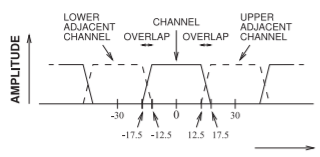
Figure \(\PageIndex{1}\): Adjacent channels showing overlap in the AMPS and DAMPS cellular systems.

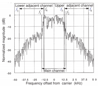
Figure \(\PageIndex{2}\): Spectrum defining adjacent channel and main channel integration limits using a \(π/4\)-DQPSK modulation scheme.

at the base station and at the mobile units.

2.11.2 Adjacent Channel Interface

Adjacent channel interference results from several factors. Since filtering is non ideal, there is inherent overlap of neighboring channels (Figure \(\PageIndex{1}\)). For this reason, adjacent channels are assigned to different cells. The nonlinear behavior of transmitters also contributes to adjacent channel interference. Thus characterization of nonlinear phenomena is important in RF design. The spectrum of a signal modulated using a QPSK scheme is shown in Figure \(\PageIndex{2}\). The signal between frequencies \(f_{1}\) and \(f_{2}\) is due to the digital modulation scheme itself. Most of the signal outside this region is due to nonlinear effects and is called spectral regrowth, a process similar to distortion of a two-tone signal. Using the frequency limits defined in Figure \(\PageIndex{2}\), the lower channel ACPR is defined as

\[\label{eq:1}\text{ACPR}_{\text{ADJ, LOWER}}=\frac{\text{Power in lower adjacent channel}}{\text{Power in main channel}}=\frac{\int_{f_{3}}^{f_{4}}X(f)df}{\int_{f_{1}}^{f_{2}}X(f)df} \]

where \(X(f)\) is the spectral power density of the RF signal. Upper channel ACPR, \(\text{ACPR}_{\text{ADJ, UPPER}}\), is similarly defined. When ACPR is being referred to without indicating whether it is upper or lower ACPR, the larger (i.e., the worse) of \(\text{ACPR}_{\text{ADJ, LOWER}}\) and \(\text{ACPR}_{\text{ADJ, UPPER}}\) is used. ACPR is usually expressed in decibels, and while the definition is such that ACPR will be less than one, when expressed in decibels, a positive number is often used (e.g., \(20\text{ dB}\) for an ACPR of \(0.01\) rather than the correct \(−20\text{ dB}\), so be careful).

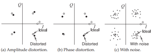
Figure \(\PageIndex{3}\): Impact of signal impairments on the constellation diagram of QPSK.

2.11.3 Noise, Distortion, and Constellation Diagrams

Noise and nonlinear distortion affect the ability to correctly demodulate signals and determine the transmitted symbols. These distortion effects can be described by their effect on the received constellation diagram, see Figure \(\PageIndex{3}\), which shows the state of the system at the sampling instant determined by the recovered carrier.

Figure \(\PageIndex{3}\)(a) shows the effect of amplitude distortion errors on the demodulated signal. Sampling of the received signal will be a distorted constellation point that does not correspond to the ideal constellation point. A decision must be made by the DSP unit as to which ideal constellation point corresponds to the distorted constellation point. The effect of phase distortion is shown in Figure \(\PageIndex{3}\)(b). Both amplitude and phase distortion could occur in the transmitter or receiver, or be the result of effects in the signal path. Figure \(\PageIndex{3}\)(c) shows the effect of noise on signal impairment. Again the constellation point extracted from the RF signal is affected by noise and the sampled and ideal constellation points do not coincide. Associating the constellation point extracted from sampling the received RF waveform with the wrong constellation point creates a symbol error and thus a bit error. Errors in recovering the carrier further distort the constellation diagram. All mobile digital radio systems adjust the level of the transmitted RF signal, and additionally in 4G and 5G cellular radio change the order of modulation, so an acceptable BER is obtained. Using more power than necessary reduces battery life and causes additional interference in other radios.

2.11.4 Comparison of GMSK and \(\pi /4\)DQPSK Modulation

This section presents the results of the type of analysis that is performed to characterize modulation methods. There is a large body of literature documenting the performance of modulation schemes and is usually the result of an assumed error model, that is the type of interference and the statistical description of that interference, and then numerical simulations. This section compares GMSK and \(π/4\)DQPSK modulation methods, the first widely-used cellular digital modulation methods.

The constellations of 4-state GMSK, see Figure 2.6.2(b), and \(π/4\)DQPSK, see Figure 2.8.8 are the same except that with \(π/4\)DQPSK the constellation rotates every closk tick. In GMSK the amplitude of the modulated carrier remains almost constant and the frequency of the carrier varies slowly. With GMSK the symbols correspond to different RF frequencies so it is not possible for symbols with frequencies at opposite ends of the frequency range to transition directly without traversing the other symbol points. This long transition results in reduction of GMSK’s modulation efficiency. With

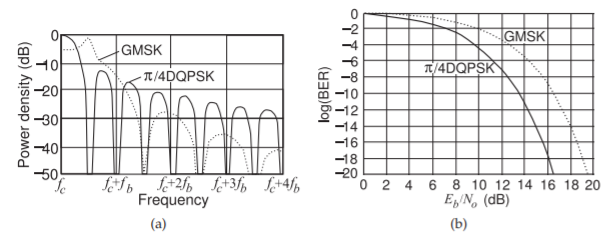
Figure \(\PageIndex{4}\): Comparison of GMSK and \(π/4\)DQPSK: (a) power spectral density as a function of frequency deviation from the carrier; and (b) BER versus signal-to-noise ratio (SNR) as \(E_{b}/N_{o}\) (or energy per bit divided by noise per bit).

\(π/4\)DQPSK there are direct transitions and the magnitude of the RF phasor does not stay constant. So while higher modulation efficiency is obtained compared to GMSK, \(π/4\)-DQPSK has a significantly time-varying envelope.

The modulation format used impacts the choice of circuitry, battery life, and the tolerance of the system to noise. Figure \(\PageIndex{4}\) contrasts the power density versus frequency and bit error rate (BER) of four-state GMSK and QPSK modulation. In Figure \(\PageIndex{4}\)(a), \(f_{c}\) is the carrier frequency and \(f_{b}\) is the bit frequency, and it is seen that GMSK and QPSK have different spectral shapes. Most of the energy is contained within the bandwidth defined by half the bit frequency (this is the symbol frequency since there are two bits per symbol). At multiples of the bit frequency, the power density with GMSK is much lower than with QPSK, resulting in less interference (adjacent channel interference [ACI]) with radios in adjacent channels. This is an important metric with radios that is captured by the adjacent channel power ratio (ACPR), the ratio of the power in the adjacent channel to the power in the main channel. Another important metric is the BER which is increased by noise in the main channel with different modulation formats differing in their susceptibility to interference. The level of noise is captured by the ratio of the power in a bit, \(E_{b}\), to the noise power, \(N_{o}\), in the time interval of a bit. This ratio, \(E_{b}/N_{o}\) (read as E B N O), is directly related to the signal-to-noise ratio (SNR). In particular, consider the plot of the BER against \(E_{b}/N_{o}\) shown in Figure \(\PageIndex{4}\)(b), where it can be seen that \(π/4\)DQPSK is less susceptible to noise than GMSK.

2.11.5 Error Vector Magnitude

The error vector magnitude (EVM) metric characterizes the accuracy of the waveform at the sampling instances and so is directly related to the BER in digital radio. EVM captures the combined effect of amplifier nonlinearities, amplitude and phase imbalances of separate \(I\) and \(Q\) signal paths, in-band amplitude ripple (e.g., due to filters), noise, non ideal mixing, non ideal carrier recovery, and DAC inaccuracies.

The EVM is a measure of the departure of a sampled phasor from the ideal

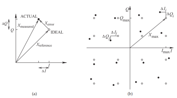
Figure \(\PageIndex{5}\): Partial constellation diagram showing quantities used in calculating EVM: (a) definition of error and reference signals; and (b) error quantities used when constellation points have different powers.

phasor located at the constellation point (see Figure \(\PageIndex{5}\)(a)). Introducing an error vector, \(X_{\text{error}}\), and a reference vector, \(X_{\text{reference}}\), that points to the ideal constellation point, the EVM is defined as the ratio of the magnitude of the error vector to the reference vector so that

\[\label{eq:2}\text{EVM}=\frac{|X_{\text{error}}|}{|X_{\text{reference}}|} \]

Expressing the error and reference in terms of the powers \(P_{\text{error}}\) and \(P_{\text{reference}}\), respectively, enables EVM to be expressed as

\[\label{eq:3}\text{EVM}=\sqrt{\frac{P_{\text{error}}}{P_{\text{reference}}}} \]

in decibels,

\[\label{eq:4}\text{EVM}_{\text{dB}}=10\log\frac{P_{\text{error}}}{P_{\text{reference}}}=20\log\frac{|X_{\text{error}}|}{|X_{\text{reference}}|} \]

or as a percentage,

\[\label{eq:5}\text{EVM}(\%)=\frac{X_{\text{error}}}{X_{\text{reference}}}\cdot 100\% \]

If the modulation format results in constellation points having different powers (e.g., with 16-QAM), the constellation point with the highest power is used as the reference and the error at each constellation point is averaged. With reference to Figure \(\PageIndex{5}\), and with \(N\) constellation points,

\[\label{eq:6}\text{EVM}=\sqrt{\frac{\frac{1}{N}\sum_{i=1}^{N}(\Delta I_{i}^{2}+\Delta Q_{i}^{2})}{X_{\text{max}}^{2}}} \]

where \(|X_{\text{max}}|\) is the magnitude of the reference vector to the most distant constellation point and \(\Delta I_{i}\) and \(\Delta Q_{i}\) are the \(I\) and \(Q\) offsets of the actual constellation point and the ideal constellation point. Note that for QAM the constellation diagram corresponds to a phasor diagram that is being continuously normalized to the average received RF signal level. In the constellation diagram the \(I\) and \(Q\) coordinates correspond to RMS quantities. Thus \(|X_{\text{max}}|\) is an RMS quantity. EVM is traditionally expressed as a percentage.

A similar measure of signal quality is the modulation error ratio (MER), a measure of the average signal power to the average error power. In decibels it is defined as

\[\label{eq:7}\text{MER}|_{\text{dB}}=10\log\frac{\frac{1}{N}\sum_{i=1}^{N}(I_{i}^{2}+Q_{i}^{2})}{\frac{1}{N}\sum_{i=1}^{N}(\Delta I_{i}^{2}+\Delta Q_{i}^{2})}=10\log\frac{\sum_{i=1}^{N}(I_{i}^{2}+Q_{i}^{2})}{\sum_{i=1}^{N}(\Delta I_{i}^{2}+\Delta Q_{i}^{2})} \]

The advantage of the MER is that it relates directly to the SNR.

Another quantity related to both the EVM and MER concepts is the implementation margin, \(k\). The implementation margin is a measure of the performance of particular hardware and is developed by design groups based on experience with similar designs. The required EVM can be estimated from the hardware implementation margin:

\[\label{eq:8}\text{EVM}_{\text{required}}=\sqrt{\frac{k}{\text{SNR}\cdot\text{PMEPR}}} \]

In decibels,

\[\label{eq:9}\text{EVM}_{\text{dB, required}}=k_{\text{dB}}-\text{SNR}_{\text{dB}}-\text{PMEPR}_{\text{dB}} \]

Example \(\PageIndex{1}\): Modulation Error Ratio

A 16-QAM modulated signal has a maximum RF phasor rms value of \(4\text{ V}\). If the noise on the signal has an rms value of \(0.1\text{ V}\), what is the modulation error ratio of the modulated signal?

Solution

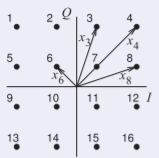
Figure \(\PageIndex{6}\)

The distance from the origin to each of the constellation points must be determined, but because of symmetry only the distances \(x_{3},\: x_{4},\: x_{7}(= x_{6})\) and \(x_{8}\) need to be calculated. The maximum RF phasor amplitude is \(4\text{ V}\), so the length \(x_{4} = 4\), with components

\[\begin{aligned}I_{4}&=Q_{4}=\sqrt{x_{4}^{2}/2}=2.828 \\ I_{6}&=\left(-\frac{1}{3}\right)\cdot I_{4}=-0.943 =-Q_{6},\text{ so }x_{6}=1.333 \\ I_{3}&=0.943;\: Q_{3}=2.828,\text{ so }x_{3}=2.981=x_{8}\end{aligned}\nonumber \]

and

\[\text{MER}=\frac{\sum_{i=1}^{16}(x_{i}^{2})}{\sum_{i=1}^{16}(x_{\text{noise}}^{2})}\nonumber \]

The calculation is simplified by considering just one quadrant and the noise, \(x_{\text{noise}} = 0.1\), is the same for each constellation point.

\[\begin{aligned}\text{MER}&=\frac{4(x_{3}^{2}+x_{4}^{2}+x_{6}^{2}+x_{8}^{2})}{16\cdot x_{\text{noise}}^{2}}\\ &=\frac{4(2.981^{2}+4^{2}+1.333^{2}+2.981^{2})}{16\cdot 0.1^{2}}=\frac{142.2}{0.16}=888.8 \\ \text{MER}|_{\text{dB}}&=10\log (888.8)=25.9\text{ dB}\end{aligned}\nonumber \]

Compare this to the SNR calculated at the individual constellation points:

\[\begin{aligned}\text{Point }3,\text{ SNR }&=x_{3}^{2}/0.1^{2}=888.6=29.5\text{ dB} \\ \text{Point }4,\text{ SNR }&=x_{4}^{2}/0.1^{2}=1600=32.0\text{ dB} \\ \text{Point }7,\text{ SNR }&=x_{7}^{2}/0.1^{2}=177.7=22.5\text{ dB}\end{aligned}\nonumber \]