4.5: Antenna Parameters

This section introduces a number of antenna metrics that are used to characterize antenna performance.

4.5.1 Radiation Density and Radiation Intensity

Antennas do not radiate equally in all directions concentrating radiated power in (usually) one direction called the main (or major) lobe of the antenna. This focusing effect is called directivity. The power in a particular direction is characterized by the radiation density and the radiation intensity metrics. The radiation density, \(S_{r}\), is the power per unit area with the SI units of \(\text{W/m}^{2}\), and will be maximum in the main lobe. Referring to Figure 4.4.1 with an antenna located at the center of the sphere of radius \(r\) and radiating a total power \(P_{r},\: S_{r}\) is the incremental radiated power \(dP_{r}\) passing through the incremental shaded region of area, \(dA\):

\[\label{eq:1}S_{r}=\frac{dP_{r}}{dA} \]

\(S_{r}\) reduces with distance falling off as \(1/r^{2}\) in free space. For a practical antenna \(S_{r}\) will vary across the surface of the sphere. The total power radiated is the closed integral over the surface \(S\) of the sphere:

\[\label{eq:2}P_{r}=\oint_{S}dP_{r}=\oint_{S}S_{r}dA \]

An alternative measure of power concentration is the radiation intensity \(U\) which is in terms of the incremental solid angle \(d\Omega\) subtended by \(dA\) so that \(d\Omega = dA/r^{2}\) and (with the SI units of \(\text{W/steradian}\) or \(\text{W/sr}\))

\[\label{eq:3}U=\frac{dP_{r}}{d\Omega}=\frac{dP_{r}}{dA}r^{2}=r^{2}S_{r} \]

Isotropic Antenna

It is useful to reference the directivity of an antenna with respect to a fictitious isotropic antenna that has no loss and radiates equally in all directions so that \(S_{r}\) is only a function of \(r\). Then integrating over the surface of the sphere yields the total radiated power

\[\label{eq:4}P_{r}|_{\text{Isotropic}}=\oint_{S}dP_{r}=\oint_{S}S_{r}dA=S_{r}\oint_{S}dA=S_{r}4\pi r^{2}=4\pi U \]

Since the isotropic antenna has no loss the power input to the antenna \(P_{\text{IN}}\) is equal to the power radiated \(P_{r} = P_{\text{IN}}\). Thus for an isotropic antenna

\[\label{eq:5} S_{r}=\frac{P_{r}}{4\pi r^{2}}=\frac{P_{\text{IN}}}{4\pi r^{2}} \]

\[\label{eq:6} U|_{\text{Isotropic}}=r^{2}S_{r}=\frac{P_{\text{IN}}}{4\pi r^{2}} \]

Antenna Efficiency

Antenna efficiency, sometimes called the radiation efficiency, describes losses in an antenna principally due to resistive (\(I^{2}R\)) losses. Resonant antennas work by creating a large current that is maximized through the generation of a standing wave at resonance. There is a lot of current, and even just a little resistance results in substantial resistive loss. The power that is reflected from the input of the antenna is usually small. The total radiated power (in all directions), \(P_{r}\), is the power input to the antenna less losses. The antenna efficiency, \(\eta_{A}\) is therefore defined as

\[\label{eq:7}\eta_{A}=P_{r}/P_{\text{IN}} \]

where \(P_{\text{IN}}\) is the power input to the antenna and \(\eta_{A} < 1\) and usually expressed as a percentage. Antenna efficiency is very close to one for many antennas, but can be \(50\%\) for microstrip patch antennas.

Antenna loss refers to the same mechanism that gives rise to antenna efficiency. Thus an antenna with an antenna efficiency of \(50\%\) has an antenna loss of \(3\text{ dB}\). Generally losses are resistive due to \(I^{2}R\) loss and mismatch loss of the antenna that occurs when the input impedance is not matched to the impedance of the cable connected to the antenna. Because of confusion with antenna gain (they are not the opposite of each other) the use of the term ‘antenna loss’ is discouraged and instead ‘antenna efficiency’ preferred.

4.5.2 Directivity and Antenna Gain

The directivity of an antenna, \(D\), is the ratio of the radiated power density to that of an isotropic antenna with the same total radiated power, \(P_{r}\):

\[\label{eq:8} D=\frac{S_{r}}{S_{r}|_{\text{Isotropic}}}=\frac{U}{U|_{\text{Isotropic}}} \]

where \(S_{r}\) and \(U\) refer to the actual antenna and the power densities and intensities are measured at the same distance from the antennas. For an actual antenna \(D\) is dependent on the direction from the antenna, see Figure \(\PageIndex{1}\). The maximum value of \(D\) will be in the direction of the main lobe of the antenna and this is called directivity gain.

The focusing property of an antenna is characterized by comparing the radiated power density to that of an isotropic antenna with the same input power. The antenna gain, \(G_{A}\), is the maximum value of \(D\) when the power input \(P_{\text{IN}} = P_{r}/\eta_{A}\) to the antenna and the isotropic antenna are the same:

\[\label{eq:9} G_{A}=\eta_{A}\text{max}(D) \]

Antenna	Type	Figure	Gain (\(\text{dBi}\))	Notes
Lossless isotropic antenna			\(0\)
\(\lambda /2\) dipole	Resonant	4.3.4(a)	\(2\)	\(R_{\text{in}}=73\:\Omega\)
\(3\lambda\) diameter parabolic dish	Traveling	—	\(38\)	\(R_{\text{in}}=\text{match}\)
Patch	Resonant	4.1.2(b)	\(9\)	\(R_{\text{in}}=\text{match}\)
Vivaldi	Traveling	4.1.2(c)	\(10\)	\(R_{\text{in}}=\text{match}\)
\(\lambda /4\) monopole on ground	Resonant	4.3.2(a)	\(2\)	\(R_{\text{in}}=36\:\Omega\)
\(5/8\lambda\) monopole on ground	Resonant	4.3.2(a)	\(3\)	Matching required

Table \(\PageIndex{1}\): Several antenna systems. \(R_{\text{in}} = \text{match}\) for resonant antennas indicates that the antenna can be designed to have an input impedance matching that of a feed cable. Traveling wave antennas are intrinsically matched.

Losses in the antenna are accounted for by the efficiency term \(\eta_{A}\).

In Equation \(\eqref{eq:9}\) \(G_{A}\) is a gain factor and is often expressed in terms of decibels (taking \(10\) times the log of \(G_{A}\)) but \(\text{dBi}\) (with ‘i’ standing for withrespect-to isotropic) is used to indicate that it is not a power gain in the same sense as amplifier gain. \(G_{A}\) instead is the ratio of power densities for two different antennas. For example, an antenna that focuses power in one direction increasing the peak radiated power density by a factor of \(20\) relative to that of an isotropic antenna has an antenna gain of \(13\text{ dBi}\). With care \(G_{A}\) can be often used in calculations of power as as with amplifier gain.

Since it is almost impossible to calculate internal antenna losses, antenna gain is invariably only measured. The input power to an antenna can be measured and the peak radiated power density, \(P_{D}|_{\text{Maximum}}\), measured in the far field at several wavelengths distant (at \(r ≫ \lambda\)). This is compared to the power density from an ideal isotropic antenna at the same distance with the same input power. Antenna gain is determined from

\[\begin{align} \label{eq:10}G_{A}&=\frac{\text{Maximum radiated power per unit area}}{\text{Maximum radiated power per unit area for an isotropic antenna}}\\ &=\frac{S_{r}|_{\text{Maximum}}}{S_{r}|_{\text{Isotropic}}} = 4\pi r^{2}\frac{P_{D}|_{\text{Maximum}}}{P_{\text{IN}}} \\ &=4\pi\frac{\text{Maximum radiated power per unit solid angle}}{\text{Total input power to the antenna}}\nonumber \\ \label{eq:11} & =4\pi\frac{(dP_{r}/d\Omega )|_{\text{Maximum}}}{P_{\text{IN}}}=4\pi r^{2}\frac{(dP_{r}/dA)|_{\text{Maximum}}}{P_{\text{IN}}}\end{align} \]

The antenna gains of common resonant and traveling-wave antennas are given in Table \(\PageIndex{1}\). In free space the antenna gain determined using Equation \(\eqref{eq:9}\) is independent of distance. Antenna gain is measured on an antenna range using a calibrated receive antenna and care taken to avoid reflections from objects, especially from the ground.

The losses of an antenna are incorporated in the antenna gain which is defined in terms of the power input to the antenna, see Equation \(\eqref{eq:11}\). Thus in calculations of radiated power using antenna gain, there is no need to separately account for resistive losses in the antenna.

In summary, antennas concentrate the radiated power in one direction so that the density of the power radiated in the direction of the peak field is higher than the power density from an isotropic antenna. Power radiated from a base station antenna, such as that shown in Figure \(\PageIndex{2}\), is concentrated in a region that looks like a toroid or, more closely, a balloon squashed at its north and south poles. Then the antenna does not radiate much power into space and will concentrate power in a region skimming the surface of

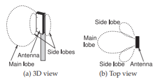
Figure \(\PageIndex{1}\): Field pattern produced by a microstrip antenna.

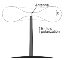
Figure \(\PageIndex{2}\): A base station transmitter pattern.

the earth. Antenna gain is a measure of the effectiveness of an antenna to concentrate power in one direction. Thus, in free space due to power spreading out the maximum power density (in SI units of \(\text{W/m}^{2}\)) at a distance \(r\) is

\[\label{eq:12}P_{D}=\frac{G_{A}P_{\text{IN}}}{4\pi r^{2}} \]

where \(4πr^{2}\) is the area of a sphere of radius \(r\) and \(P_{\text{IN}}\) is the input power.

Measurements of antenna gain are used to derive antenna efficiency. It is impossible to measure or simulate the resistive and dielectric losses of an antenna directly. Antenna efficiency is obtained using theoretical calculations of antenna gain assuming no losses in the antenna itself. This is compared to the measured antenna gain yielding the antenna efficiency.

Example \(\PageIndex{1}\): Antenna Gain

A base station antenna has an antenna gain, \(G_{A}\), of \(11\text{ dBi}\) and a \(40\text{ W}\) input. The transmitted power density falls off with distance \(d\) as \(1/d^{2}\). What is the peak power density at \(5\text{ km}\)?

Solution

A sphere of radius \(5\text{ km}\) has an area \(A = 4πr^{2} = 3.142\cdot 10^{8} m^{2};\: G_{A} = 11\text{ dBi} = 12.6\). In the direction of peak radiated power, the power density at \(5\text{ km}\) is

\(P_{D}=\frac{P_{\text{IN}}G_{A}}{A}=\frac{40\cdot 12.6\text{ W}}{3.142\cdot 10^{8}\text{ m}^{2}}=1.603\:\mu\text{W/m}^{2}\)

Example \(\PageIndex{2}\): Antenna Efficiency

A antenna has an antenna gain of \(13\text{ dBi}\) and an antenna efficiency of \(50\%\) and all of the loss is due to resistive losses and resistance of metals is proportional to temperature. The RF signal input to the antenna has a power of \(40\text{ W}\).

1. What is the input power in dBm?
   \(P_{\text{in}} = 40\text{ W} = 46.02\text{ dBm}\).
2. What is the total power transmitted in \(\text{dBm}\)?
   \[\begin{aligned}P_{\text{Radiated}} = 50\%\text{ of }P_{\text{IN}} &= 20\text{ W}\text{ or }43.01\text{ dBm.}\nonumber\\ \text{Alternatively, }P_{\text{Radiated}} &= 46.02\text{ dBm} − 3\text{ dB} = 43.02\text{ dBm.}\nonumber\end{aligned} \nonumber \]
3. If the antenna is cooled to near absolute zero so that it is lossless, what would the antenna gain be?
   The antenna gain would increase by \(3\text{ dB}\) and antenna gain incorporates both directivity and antenna losses. So the gain of the cooled antenna is \(16\text{ dBi}\).

4.5.3 Effective Isotropic Radiated Power

A transmit antenna does not radiate power equally in all directions and for a receiver in the main lobe of the transmit antenna it is as though there is an isotropic transmit antenna with a much higher input power. This concept is incorporated in the effective isotropic radiated power (EIRP):

\[\label{eq:13} \text{EIRP}=P_{\text{IN}}G_{A} \]

This uses antenna gain to derive the total power that would be radiated by an isotropic antenna producing the same (peak) power density as the actual antenna. Regulatory limits on the power levels of transmitters are in terms of EIRP rather than the total radiated power. Sometimes equivalent radiated power (ERP) is used instead of EIRP with the same meaning.

4.5.4 Effective Aperture Size

Effective aperture size is defined so that the power density at a receive antenna when multiplied by its effective aperture size, \(A_{R}\), yields the power output from the antenna at its connector. Since antennas are linear and reciprocal it is is to be expected that there is a relationship between effective aperture size and antenna gain.

An antenna has an effective size that is more than its actual physical size. This is because of its influence on the EM fields around it. The power captured by an antenna is the effective aperture size (or area) multiplied by the transmitted power density. That is, the effective aperture size of an antenna is the area of the surface that captures all of the power passing through it and delivers this power to the output terminals of the antenna.

The effective aperture area of a receive antenna, \(A_{R}\), is related to the receive antenna gain, \(G_{R}\), as follows [2, 3] (note that \(A_{e}\) is often used if it is not necessary to distinguish antennas):

\[\label{eq:14}A_{R}=\frac{G_{R}\lambda ^{2}}{4\pi} \]

where \(\lambda\) is the wavelength of the radio signal\(^{1}\). The effective aperture area of an antenna can have little to do with its physical size; e.g., a wire antenna has almost no physical size but has a significant effective aperture size.

If \(S_{r}\) is the transmitted power density at the receive antenna, the power received is

\[\label{eq:15}P_{R}=P_{D}A_{R}=P_{D}\frac{G_{R}\lambda ^{2}}{4\pi} \]

Here \(P_{R}\) is the power delivered at the output connector of the receive antenna, as loss in the receive antenna is incorporated in \(G_{R}\) and \(A_{R}\). The total power radiated by the transmit antenna in the direction of maximum power density is given by multiplying the power input to the transmit antenna, \(P_{T}\),\(^{2}\) by the antenna gain of the transmit antenna, \(G_{T}\). This can be converted to the power density at a distance \(d\) (ignoring multipath effects),

\[\label{eq:16}S_{r}=\frac{P_{T}G_{T}}{4\pi d^{2}} \]

and the power delivered by the receive antenna is

\[\label{eq:17}P_{R}=S_{r}A_{R}=\frac{P_{T}G_{T}}{4\pi d^{2}}\frac{G_{R}\lambda ^{2}}{4\pi}=P_{T}G_{T}G_{R}\left(\frac{\lambda}{4\pi d}\right)^{2} \]

That is,

\[\label{eq:18}P_{R}=P_{T}G_{T}G_{R}\left(\frac{\lambda}{4\pi d}\right)^{2} \]

This equation is known as the Friis transmission equation or the Friis transmission formula.

Equation \(\eqref{eq:18}\) provides a powerful tool for evaluating the power received in a communication system and modifications have been developed to account for impairments that are encountered. One of the assumptions in the development of Equation \(\eqref{eq:18}\) is that the polarization of the receive antenna matches that of the transmitted signal. The transmit antenna will radiate a signal with an electric field with a particular polarization, i.e. \(E\) field orientation. Propagation through air has little effect on the polarization of a signal, although atmospheric conditions can rotate the polarization slightly. A polarization mismatch factor could be included in Equation \(\eqref{eq:18}\). For ground-based communications, such as cellular communications, reflections and diffraction have a major impact on the power of the received signal and techniques for handling these effects are considered in the next section.

4.5.5 Summary

This section introduced several metrics for characterizing antennas:

\(\begin{array}{lllll}{\text{Metric}}&{\quad}&{\text{Equation}}&{\quad}&{\text{Description}}\\{S_{r}}&{\quad}&{\eqref{eq:1}}&{\quad}&{\text{Radiated power density, W/m}^{2}} \\ {U}&{\quad}&{\eqref{eq:3}}&{\quad}&{\text{Radiation intensity W/sr}} \\{\eta_{A}}&{\quad}&{\eqref{eq:14}}&{\quad}&{\text{Antenna efficiency}}\\{D}&{\quad}&{\eqref{eq:8}}&{\quad}&{\text{Antenna directivity}}\\{G_{A}}&{\quad}&{\eqref{eq:10}}&{\quad}&{\text{Antenna gain, used with a transmit antenna}}\\{A_{e}}&{\quad}&{\eqref{eq:14}}&{\quad}&{\text{Effective aperture area, used with a receive antennaa}}\\{\text{EIRP}}&{\quad}&{\eqref{eq:13}}&{\quad}&{\text{Equivalent isotropic radiated power}}\end{array}\)

Example \(\PageIndex{3}\): Point-to-Point Communication

In a point-to-point communication system, a parabolic receive antenna has an antenna gain of \(60\text{ dBi}\). If the signal is \(60\text{ GHz}\) and the power density at the receive antenna is \(1\text{ pW/cm}^{2}\), what is the power at the output of the receive antenna connected to the RF electronics?

Solution

The first step is determining the effective aperture area, \(A_{R}\), of the parabolic antenna. The frequency is \(60\text{ GHz}\), and so the wavelength (\(\lambda\)) is \(5\text{ mm}\). Also note that \(G_{R}=60\text{ dBi}=10^{6}\). From Equation \(\eqref{eq:14}\)

\[\label{eq:19}A_{R}=\frac{G_{R}\lambda ^{2}}{4\pi}=\frac{10^{6}\cdot 0.005^{2}}{4\pi}=1.989\text{ m}^{2} \]

Using Equation \(\eqref{eq:15}\) \(P_{D} = 1\text{ pW/cm}^{2} = 10\text{ nW/m}^{2}\), the total power delivered to the RF receiver electronics (at the output of the receive antenna) is

\[\label{eq:20}P_{R}=P_{D}A_{R}=10\text{ nW}\cdot\text{m}^{-2}\cdot 1.989\text{ m}^{2}=19.89\text{ nW} \]

Footnotes

[1] The derivation of Equation \(\eqref{eq:14}\) invokes a thought experiment with an antenna connected to a resistor in thermal equilibrium and each in separate thermally isolated chambers with black body walls [4, 5]. The available thermal (Johnson-Nyquist) noise power from the resistor is radiated by the antenna (incorporating antenna gain) and absorbed by the walls of the antenna’s chamber. The same amount of power, as black body radiation from the walls of the antenna’s chamber, must be received by the antenna (incorporating effective aperture size) and delivered to the resistor where it is dissipated as heat. At frequencies up to infrared and at room temperature (and hence at radio frequencies) the power density of black body radiation increases linearly with temperature and as the square of frequency (i.e. as \(1/\lambda^{2}\)) whereas Johnson-Nyquist noise is independent of frequency but increases linearly with temperature. The derivation is exact for an isotropic antenna and assumed to apply to all antennas.

[2] Note that this was \(P_{\text{IN}}\) previously and here the subscript \(T\) is used to indicate the power input to the transmit antenna.