5.10: Radar Systems

Radar uses EM signals to determine the range, altitude, direction, and speed of objects called targets by looking at the signals received from transmitted signals called radar waveforms. Common radar bands and applications are given in Table \(\PageIndex{1}\). The earliest use of EM signals to detect targets was demonstrated in 1904 by Christian Hulsmeyer using a spark gap generator [39]. This system was promoted as a system to avoid collisions of ships and detected the direction of targets only. Research contributed to further developments, with a significant acceleration during World War II. Radar is now a word in its own right, but in 1941 the term RADAR was created as an acronym for radio detection and ranging.

Band	Frequency	Wavelength	Application
HF	\(3-30\text{ MHz}\)	\(10-100\text{ m}\)	Over-the-horizon radar, oceanographic mapping
VHF	\(30-300\text{ MHz}\)	\(1-10\text{ m}\)	Oceanographic mapping, atmospheric monitoring, long-range search
UHF	\(0.3-1\text{ GHz}\)	\(1\text{ m}-30\text{ cm}\)	Long-range surveillance, foliage penetration, ground penetration, atmospheric monitoring
L	\(1–2\text{ GHz}\)	\(15–30\text{ cm}\)	Satellite imagery, mapping, long-range surveillance, environmental monitoring
S	\(2-4\text{ GHz}\)	\(7.5–15\text{ cm}\)	Weather radar, air traffic control, surveillance, search, IFF (identify, friend or foe)
C	\(4–8\text{ GHz}\)	\(3.75–7.5\text{ cm}\)	Hydrological radar, topography, fire control, weather
X	\(8–12\text{ GHz}\)	\(2.5–3.75\text{ cm}\)	Cloud radar, air-to-air missile seeker, maritime, air turbulence, police radar, high-resolution imaging, perimeter surveillance
Ku	\(12–18\text{ GHz}\)	\(1.7–2.5\text{ cm}\)	Remote sensing, short-range fire control, perimeter surveillance; pronounced “kay-you”
K	\(12=8–27\text{ GHz}\)	\(1.2–1.7\text{ cm}\)	Police radar, remote sensing, perimeter surveillance
Ka	\(27–40\text{ GHz}\)	\(7.5–12\text{ mm}\)	Police radar, weapon guidance, remote sensing, perimeter surveillance, weapon guidance; pronounced “kay-a”
V	\(40–75\text{ GHz}\)	\(4–7.5\text{ mm}\)	Perimeter surveillance, remote sensing, weapon guidance
W	\(75-110\text{ GHz}\)	\(2.7-4\text{ mm}\)	Perimeter surveillance, remote sensing, weapon guidance

Table \(\PageIndex{1}\): IEEE radar bands and applications.

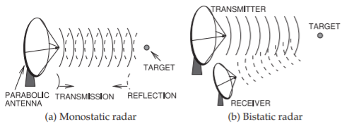
Figure \(\PageIndex{1}\): Radar system: (a) monostatic radar with the same site used for transmission of the radar signal and receipt of the reflection from the target; and (b) bistatic radar with different transmit and receive sites.

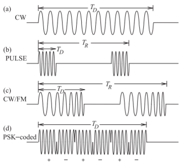
Figure \(\PageIndex{2}\): Radar waveforms: (a) continuous wave; (b) pulsed wave; (c) frequency modulated continuous wave; and (d) phase-encoded (PSK-coded) waveform.

In a radar system, typically a high-gain antenna such as a parabolic antenna is used to transmit a radar signal, but always a high-gain antenna is used to receive the signal. If the same antenna is used for transmit and receive (possibly two similar antennas at the same site) the system is called a monostatic radar (see Figure \(\PageIndex{1}\)(a)). Radar with transmit and receive antennas at different sites is called bistatic radar (shown in Figure \(\PageIndex{1}\)(b)).

In a monostatic radar using the same antenna for transmit and receive, the space is painted with a radar signal and the received signal is captured after a propagation delay from the antenna to the target and back again. A radar image can then be developed. In many radars the receive antenna is mechanically steered and often a regular rotation is used. With so-called synthetic aperture radars, a platform such as an aircraft moves the radar in one direction and a one-dimensional mechanical or electrical scan enables a two-dimensional image to be developed.

The categories of radar waveforms are shown in Figure \(\PageIndex{2}\). The continuous wave (CW) waveform shown in Figure \(\PageIndex{2}\)(a) is on all or most of the time and is used to detect a reflection from a target. This reflected signal is much smaller than the transmitted signal and it can be difficult to separate the transmitted and received signals. A monostatic CW radar architecture is shown Figure \(\PageIndex{3}\)(a), where a circulator\(^{1}\) is used to separate the transmitted and received signals. The received signal is converted to digital form using

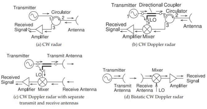
Figure \(\PageIndex{3}\): Radar architectures.

an ADC and the bandwidth of the ADC with the required dynamic range determines the limit on the bandwidth of the radar signal. Generally the broader the bandwidth, the better the radar system is at identifying objects. A CW signal can be used to develop an image, but it is not good at determining the range of a target. For this, a pulsed radar waveform, as shown in Figure \(\PageIndex{2}\)(b), is better. The repetition period, \(T_{R}\), is more than the round-trip time to the target, thus the time interval between the transmitted signal and the returned signal can be used to estimate range. Direction is determined by the orientation of the antenna.

The CW architecture can also be used with pulsed radar. In pulsed radar, the signal received contains the desired target signal, multipath and echoes, and clutter, as shown in Figure \(\PageIndex{4}\)(a). These effects also appear in the signal received in CW radar, but it is much easier to see in pulsed radar. Identifying clutter and multipath effects is a major topic in radar processing. Alternative waveforms, especially digitally modulated waveforms, aid in extracting the desired information. The frequency modulated waveform, or chirp waveform, in Figure \(\PageIndex{2}\)(c), will have a reflection that will also be chirped, and the difference between the frequency being transmitted and that received indicates the range of the target, provided that the target is not moving. The radar architecture that can be used to extract this information is shown in Figure \(\PageIndex{3}\)(b). The directional couplers tap off a small part of the transmit signal and use it as the LO of a mixer with the received signal as input. A similar architecture is shown in Figure \(\PageIndex{3}\)(c), but now separate transmit and receive antennas are used to separate the transmitted and received signals rather than using a circulator. Better separation of the transmitted and received signals can be obtained this way. The frequency of the IF that results is proportional to the range of the target.

An important concept in radar is that of radar cross section (RCS) denoted \(\sigma\) (with SI units of \(\text{m}^{2}\)). The RCS of a target is the equivalent area that

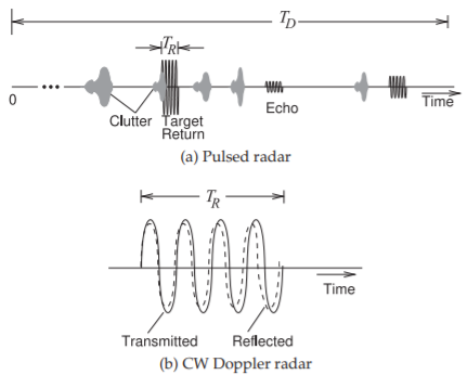
Figure \(PageIndex{4}\): Radar returns. The strength of the reflected signal depends on the radar cross section (RCS), \(\sigma\), of the target. \(\sigma = 0.01\text{ m}^{2}\) for a bird, \(< 0.1\text{ m}^{2}\) for a stealth aircraft, \(1\text{ m}^{2}\) for a human, \(2– 6\text{ m}^{2}\) for a conventional fighter plane, \(100\text{ m}^{2}\) for a large commercial aircraft, \(200\text{ m}^{2}\) for a truck, \(10,000–100,000\text{ m}^{2}\) for a container ship.

intercepts the power of a transmitted signal and re-radiates all of that power isotropically to produce the observed power density at a receiver [40]. The RCS therefore depends on the frequency of the transmitted signal, the size of the target, the incident and reflected angle of the signal reflected by the target, and the reflectivity of the target.

The power of the signal reflected by the target and captured by the receive antenna is given by the radar equation [40]:

\[\label{eq:1}P_{R}=\frac{P_{T}G_{T}A_{R}\sigma F^{4}}{(4\pi )^{2}R_{T}^{2}R_{R}^{2}} \]

where \(P_{T}\) is the transmit power delivered to the transmit antenna, \(G_{T}\) is the antenna gain of the transmitter, \(A_{R}\) is the effective aperture area of the receive antenna, \(F\) is the pattern propagation factor, \(R_{T}\) is the distance from the transmitter to the target, and \(R_{R}\) is the distance from the target to the receiver. \(F\) captures the effective loss due to multipath, which was captured in communications by introducing a signal dependence of \(1/d^{n}\), where \(n\) ranges from \(2\) to \(4\) depending on the environment. In free space, \(F = 1\). If the same antenna is used for transmit and receive, and multipath is not important (so \(F = 1\)), then Equation \(\eqref{eq:1}\) becomes

\[\label{eq:2}P_{R}=\frac{P_{T}G_{T}A_{R}\sigma}{(4\pi )^{2}R^{4}} \]

where \(R = R_{T} = R_{R}\). In Section 4.5.4 the antenna effective area was related to the antenna gain. From Equation (4.5.14),

\[\label{eq:3}A_{R}=\frac{G_{r}\lambda^{2}}{4\pi} \]

and so, with \(G_{R} = G_{T}\), Equation \(\eqref{eq:2}\) becomes

\[\label{eq:4}P_{R}=\frac{P_{T}G_{T}^{2}\lambda^{2}\sigma}{(4\pi)^{3}R^{4}} \]

Radar frequency, \(f_{T}\)	Relative speed, \(v_{R}\)
	\(1\text{ m/s}\)	\(100\text{ km/hr}\)	\(1000\text{ km/hr}\)
\(500\text{ MHz}\)	\(3.3\text{ Hz}\)	\(92.6\text{ Hz}\)	\(925.9\text{ kHz}\)
\(2\text{ GHz}\)	\(13.3\text{ Hz}\)	\(370.4\text{ Hz}\)	\(3.704\text{ kHz}\)
\(10\text{ GHz}\)	\(66.7\text{ Hz}\)	\(1.852\text{ kHz}\)	\(18.519\text{ kHz}\)
\(40\text{ GHz}\)	\(266.7\text{ Hz}\)	\(7.407\text{ kHz}\)	\(74.074\text{ kHz}\)

Table \(\PageIndex{2}\): Doppler frequency shifts for targets moving toward a radar at speed \(v_{R}\).

If a signal of frequency \(f_{T}\) is transmitted and reflected from a moving target there is a Doppler shift, \(f_{D}\), and the received signal will be at frequency

\[\label{eq:5}f_{R}=f_{T}+f_{D}\quad\text{(target moving toward the radar)} \]

\[\label{eq:6}f_{R}=f_{T}-f_{D}\quad\text{(target moving away from the radar)} \]

where

\[\label{eq:7}f_{D}=2v_{R}f_{T}/c \]

In Equation \(\eqref{eq:6}\) \(v_{R}\) is the radial component of the speed of the target relative to the radar, and \(c\) is the speed of light. Typical Doppler shifts are shown in Table \(\PageIndex{2}\).

If the target is moving, there will be a Doppler shift. If the target is moving toward a CW radar, then the frequency of the returned signal will be higher, as shown in Figure \(\PageIndex{4}\)(b). A similar architecture to that used with chirp radar can be used (see Figures \(\PageIndex{3}\)(bc)). The concept can be extended to bistatic radars, but now the local oscillator reference must be generated. As was seen previously, the frequency of the transmit carrier can be recovered for digitally modulated signals such as the PSK-encoded signals shown in Figure \(\PageIndex{2}\)(d). Advanced high-end radars use digital modulation and CDMA-like waveforms and exploit space-time coding. Typically the radar waveforms to be transmitted are chirped, which is a technique that takes the desired transmit waveform and stretches it out in time so that it can be more efficiently amplified and more power can be transmitted. At the receiver, the radar signal is compressed in time so that it corresponds to the original transmit signal prior to chirping.

It should be apparent that radars and radar waveforms can be optimized for imaging or for exploiting Doppler shifts to track moving targets. Imaging is suitable when there is little clutter, such as looking into the air. However, it is difficult to detect targets such as cars that are moving on the ground. So-called ground moving target indication (GMTI) radar relies on Doppler shifts to discriminate moving targets, and then the ability to image accurately is compromised. Considerable effort is devoted to developing waveforms that are difficult to detect (stealthy) and are optimized for imaging or GMTI.

Footnotes

[1] For the circulator shown, power entering port 1 of a circulator leaves at port 2 and power entering port 2 is delivered to port 3. So ports 1 and 3 are isolated.