1.1: Introduction to Amplifiers and Oscillators

Design of microwave amplifiers and oscillators is the most challenging of microwave designs determining the performance and DC power consumption of microwave systems. Most of the challenges arise because of the capacitive parasitics of microwave transistors and also because some types of transistors, such as silicon transistors, have quite low intrinsic power gain. Packaged transistors which are used in hybrid design and design using modules have the additional complexity of package inductance as well as additional capacitance from the package. With amplifiers one of the great challenges is achieving wide bandwidth so that the same amplifier can be used for multiple frequency bands. For example, with cellular communications it is desirable if one amplifier could be used for multiple cellular bands. However most of the time a cellular system handset must have different transmit and receive amplifiers for each of the cellular bands. The transistor’s capacitive, and if packaged inductive, parasitics determine the minimum \(Q\) and thus maximum bandwidth. The matching required to interface the input and the of an amplifier output of transistors can only further reduce bandwidth.

Microwave amplifier design generally uses the topology shown in Figure \(\PageIndex{1}\) with the transistor biased in a high-gain region and the input and output matching networks used to provide good power transfer at the input and output of the transistors. The DC bias control circuit is fairly standard; it does not involve any microwave constraints other than the need to block RF currents from the bias circuit. The lowpass filters (in the bias circuits) can have one of several forms and are often integrated into the input and output matching networks. Synthesis of the input and output matching networks (and occasionally a feedback network required for stability and broadband operation) is the primary objective of any amplifier design.

Design of linear microwave amplifiers where narrowband operation is

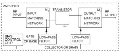
Figure \(\PageIndex{1}\): Block diagram of an RF amplifier including biasing networks.

sufficient is considered in Chapter 2 where the topology shown in Figure \(\PageIndex{1}\) is nearly always followed. The input and output matching networks limit the bandwidth of the amplifier and are ideally lossless. This chapter develops the skills required to trade off gain, noise, and stability. These trade-offs are required with all types of microwave amplifier design. The chapter presents a case study of narrowband linear amplifier design.

Chapter 3 presents strategies for designing a wideband amplifier and again the topology shown in Figure \(\PageIndex{1}\) is usually followed. Wideband is still limited as usually the best that can be achieved for an efficient amplifier is a bandwidth of only half-an-octave such as a bandwidth from \(2\) to \(3\text{ GHz}\). Sometimes there is inductive and capacitive feedback around the transistor to compensate for the inherent gain roll-off with respect to frequency of transistors, especially FETs. The chapter includes a case study on the design of a wideband amplifier. A case study is a good way to present design methods as it enables design decisions to be discussed. Rarely can design decisions be reduced to a formulaic flow. One of the important trade-offs is trading off gain and noise performance and in the case study it will be seen how this can be done graphically. A distributed amplifier is one type of amplifiers that has a very wide bandwidth, perhaps \(2–4\) octaves, e.g. \(2\) to \(4\text{ GHz}\) or \(2\) to \(16\text{ GHz}\), but has an efficiency of only a few percent. The topology differs significantly from the input and output matching network–based topology of Figure \(\PageIndex{1}\). The distributed amplifier achieves wide bandwidth by incorporating the parasitics of multiple transistors in a transmission line where the input and output capacitances of transistors augment the capacitances in the \(LC\) model of an actual transmission line. A case study is presented that analyses a distributed amplifier. Efficient biasing of a wideband amplifier can be a challenge and a final case study presents a technique for distributed biasing of a differential amplifier.

The fourth chapter considers power amplifiers where the emphasis is on producing large powers at high efficiency and bandwidth is sacrificed. Usually at high powers efficiencies are achieved by engineering the transistor’s current and voltage waveforms by manipulating the impedances presented at harmonics. This is the source of the low bandwidth. A case study of the design of a WiMAX power amplifier is undertaken.

The final chapter of this book considers the design of microwave oscillators. Microwave oscillator design is particularly challenging. Oscillators consume considerable DC power and are a competitive differentiator. There are two quite different classes of design, one for oscillators that are fixed in frequency and one for the much more useful voltage-controlled oscillator which has variable frequency. Case studies are presented for each of these two types of oscillators.

The remainder of this current chapter describes transistor technology and an appendix describes particular models of transistors that are used in circuit simulators. Today’s simulators use transistor models that are very sophisticated compared to those models described in the appendix, however they are not amenable to developing a designer’s intuition. The simpler models considered in the appendix, state-of-the-art models from \(20\) and \(30\) years ago, provide the desired intuition for a designer.