2.6: Amplifier Stability

The potential exists for an amplifier to be unstable and oscillate. Generally this is not a constant oscillation with fixed amplitude and frequency, but a chaotic response. Oscillator design is not as simple as designing an unstable amplifier, if only one could be so lucky. There is not a simple metric that will indicate whether an amplifier will be stable or not. In the worst case a transistor will oscillate no matter what is done to the external circuitry [10]. A manufacturer could not sell such a transistor and it would not be a useful component in a monolithic integrated process. So it is not surprising that stable amplifiers can be designed using available transistors. For stability analysis, the active device in a linear amplifier can often be treated as a two-port (see Figure 2.5.6(a)).

Stability considerations affect the maximum (stable) gain that can be achieved and the ease of design. If the maximum stable gain is too low then another transistor needs to be selected. If the specified gain is close to the maximum stable gain, then design will be challenging, especially for broader bandwidths. So design effort increases with simpler (and hence cheaper) transistors. Experience is the best guide to making this tradeoff.

There are many ways of looking at stability. In the time-domain instability is manifested as the growth of signals over time independent of the level of the input signal. However it is most efficient to analyze and design RF and microwave circuits in the frequency domain and so stability must be assessed in the frequency domain as well. The many frequency domain techniques available to assess stability vary by the level of coverage and ease by which they can be applied. The simplest and most easily applied technique is based on two-port analysis, which leads to stability metrics based on two-port \(S\) parameters and to the concept of regions (called circles) of stability on a Smith chart and a more general technique is Nyquist stability analysis. These are considered below.

2.6.1 Two-Port Stability Analysis

Stability analysis should be applied to the innermost two-port containing the active device and any feedback networks. If the innermost two-port (including any feedback) is unconditionally stable, then the amplifier in which it is embedded will be stable. Thus there is a natural selection process so that available transistors tend to not suffer from internal instabilities.

Oscillation will initiate if signals reflected at the input port increase in amplitude as the signal reflects first from the source, \(\Gamma_{S}\), and then from the input port. That is, if

\[\label{eq:1}|\Gamma_{S}\Gamma_{\text{IN}}|>1 \]

the amplifier will be potentially unstable at the input. Whether or not it is actually unstable will depend on the phases of \(\Gamma_{S}\) and \(\Gamma_{\text{IN}}\). This situation is shown in the signal flow graph of Figure 2.5.6(b), where oscillation is initiated by noise. Similarly oscillation will occur if multiple reflections between the output and the load build in amplitude. That is, if

\[\label{eq:2}|\Gamma_{L}\Gamma_{\text{OUT}}|>1 \]

with the oscillation initiated by noise as shown in Figure 2.5.6(c). Now

\[\label{eq:3}|\Gamma_{\text{IN}}|=\left|S_{11}+\frac{S_{12}S_{21}\Gamma_{L}}{1-S_{22}\Gamma_{L}}\right| \]

and

\[\label{eq:4}|\Gamma_{\text{OUT}}|=\left|S_{22}+\frac{S_{12}S_{21}\Gamma_{S}}{1-S_{11}\Gamma_{S}}\right| \]

Combining Equations \(\eqref{eq:1}\)–\(\eqref{eq:4}\), the amplifier will be unstable if

\[\label{eq:5}|\Gamma_{S}\Gamma_{\text{IN}}|=\left|\Gamma_{S}S_{11}+\frac{S_{12}S_{21}\Gamma_{S}\Gamma_{L}}{1-S_{22}\Gamma_{L}}\right|>1 \]

or

\[\label{eq:6}|\Gamma_{L}\Gamma_{\text{OUT}}|=\left|\Gamma_{L}S_{22}+\frac{S_{12}S_{21}\Gamma_{S}\Gamma_{L}}{1-S_{11}\Gamma_{S}}\right|>1 \]

The coupling of \(\Gamma_{S}\) and \(\Gamma_{L}\) makes it difficult to independently design the input and output matching networks. It is much more convenient to consider the unconditionally stable situation whereby the input is stable no matter what the load and output matching network present, and the output is stable no matter what the source and input matching network present. As a first stage in design, a linear amplifier is designed for unconditional stability. The design space is larger if the more rigorous test for stability, embodied in Equations \(\eqref{eq:5}\) and \(\eqref{eq:6}\), is used to determine stability. The advantage (i.e., a larger design space), however, is often small.

If the source and load are passive, then \(|\Gamma_{S}| < 1\) and \(|\Gamma_{L}| < 1\) so that oscillations will build up if

\[\label{eq:7}|\Gamma_{\text{IN}}|>1\quad\text{and}\quad |\Gamma_{\text{OUT}}|>1 \]

For guaranteed stability for all passive source and load terminations (i.e., unconditional stability), then

\[\label{eq:8}|\Gamma_{\text{IN}}|<1\quad\text{and}\quad |\Gamma_{\text{OUT}}|<1 \]

Amplifiers are often realized as stages whereby one amplifier stage feeds another. This complicates stability analysis, as it is possible for \(\Gamma_{S}\) and \(\Gamma_{L}\) to be more than unity. If \(\Gamma_{S}\) and \(\Gamma_{L}\) are both less than one for multiple amplifier stages, then the amplifier stability being described here can be used.

For the stability criteria to be used in design they must be put in terms of the scattering parameters of the active device. There are two suitable stability criteria commonly used, the \(k\)-factor and the \(\mu\)-factor, which will now be considered.

2.6.2 Unconditional Stability: Two-Port Stability Circles

The input reflection coefficient of an active device is determined by the \(S\) parameters of the device and the load:

\[\label{eq:9}\Gamma_{\text{IN}}=S_{11}+\frac{S_{12}S_{21}\Gamma_{L}}{1-S_{22}\Gamma_{L}} \]

and so for stability (for \(|\Gamma_{S}| \leq 1\))

\[\label{eq:10}|\Gamma_{\text{IN}}|=\left|S_{11}+\frac{S_{12}S_{21}\Gamma_{L}}{1-S_{22}\Gamma_{L}}\right|<1 \]

Similarly, considering the output of the active device, for stability (with \(|\Gamma_{L}|\leq 1\)),

\[\label{eq:11}|\Gamma_{\text{OUT}}|=\left|S_{22}+\frac{S_{12}S_{21}\Gamma_{S}}{1-S_{11}\Gamma_{S}}\right|<1 \]

Equations \(\eqref{eq:10}\) and \(\eqref{eq:11}\) must hold for all

\[\label{eq:12}|\Gamma_{S}|\leq 1\quad\text{and}\quad |\Gamma_{L}|\leq 1 \]

When the active is unilateral, \(S_{12} = 0\), and Equations \(\eqref{eq:10}\) and \(\eqref{eq:11}\) simplify to the requirement that \(|S_{11}| < 1\) and \(|S_{22}| < 1\). Otherwise, given a device, there will be a limit on the values of \(\Gamma_{S}\) and \(\Gamma_{L}\) that will ensure stability. The stability criteria are in terms of the magnitudes of complex numbers, and this is known to specify circles in the complex plane. The following development will lead to the center and radius defining the stability circles that define the boundaries between stable and potentially unstable regions.

For \(|\Gamma_{\text{IN}}| = 1\), the output stability circle is defined by

\[\label{eq:13}\left|S_{11}+\frac{S_{12}S_{21}\Gamma_{L}}{1-S_{22}\Gamma_{L}}\right|=1 \]

The development that follows puts this into the standard form for a circle, that is, in the form of

\[\label{eq:14}|\Gamma_{L}-c|=r \]

where \(c\) is a complex number and defines the center of the circle on a reflection coefficient plot, and \(r\) is a real number and is the radius of the circle. This circle defines the boundary between stable and potentially unstable values of \(\Gamma_{L}\). Now Equation \(\eqref{eq:13}\) can be rewritten as

\[\label{eq:15}|S_{11}-(S_{11}S_{22}-S_{12}S_{21})\Gamma_{L}|=|1-S_{22}\Gamma_{L}| \]

which includes the determinant, \(\Delta\), of the scattering parameter matrix. With

\[\label{eq:16}\Delta=S_{11}S_{22}-S_{12}S_{21} \]

Equation \(\eqref{eq:15}\) becomes

\[\label{eq:17}|S_{11}-\Delta\Gamma_{L}|=|1-S_{22}\Gamma_{L}| \]

Removing the absolute signs by multiplying each side by its complex conjugate and then rearranging,

\[\begin{align}\label{eq:18}(S_{11}-\Delta\Gamma_{L})(S_{11}-\Delta\Gamma_{L})^{\ast}&=(1-S_{22}\Gamma_{L})(1-S_{22}\Gamma_{L})^{\ast} \\ \label{eq:19}S_{11}S_{11}^{\ast}+\Delta\Delta^{\ast}\Gamma_{L}\Gamma_{L}^{\ast}-(\Delta\Gamma_{L}S_{11}^{\ast}+\Delta^{\ast}\Gamma_{L}^{\ast}S_{11})&=1+S_{22}S_{22}^{\ast}\Gamma_{L}\Gamma_{L}^{\ast} -(S_{22}\Gamma_{L}+S_{22}^{\ast}\Gamma_{L}^{\ast}) \\ \label{eq:20}\left(|S_{22}|^{2}-|\Delta|^{2}\right)\Gamma_{L}\Gamma_{L}^{\ast}-(S_{22}-\Delta S_{11}^{\ast})\Gamma_{L}-(S_{22}^{\ast}-\Delta ^{\ast}S_{11})\Gamma_{L}^{\ast}&=|S_{11}|^{2}-1 \\ \label{eq:21}\Gamma_{L}\Gamma_{L}^{\ast}-\frac{(S_{22}-\Delta S_{11}^{\ast})\Gamma_{L}}{|S_{22}|^{2}-|\Delta |^{2}}-\frac{(S_{22}-\Delta S_{11}^{\ast})^{\ast}\Gamma_{L}^{\ast}}{|S_{22}|^{2}-|\Delta |^{2}}&=\frac{|S_{11}|^{2}-1}{|S_{22}|^{2}-|\Delta |^{2}} \end{align} \]

Adding the same term to both sides,

\[\begin{align}\Gamma_{L}\Gamma_{L}^{\ast}&-\frac{(S_{22}-\Delta S_{11}^{\ast})\Gamma_{L}}{|S_{22}|^{2}-|\Delta |^{2}}-\frac{(S_{22}-\Delta S_{11}^{\ast})^{\ast}\Gamma_{L}^{\ast}}{|S_{22}|^{2}-|\Delta |^{2}}+\frac{(S_{22}-\Delta S_{11}^{\ast})(S_{22}-\Delta S_{11}^{\ast})^{\ast}}{\left(|S_{22}|^{2}-|\Delta |^{2}\right)^{2}} \nonumber \\ \label{eq:22}&=\frac{|S_{11}|^{2}-1}{|S_{22}|^{2}-|\Delta |^{2}}+\frac{(S_{22}-\Delta S_{11}^{\ast})(S_{22}-\Delta S_{11}^{\ast})^{\ast}}{\left(|S_{22}|^{2}-|\Delta |^{2}\right)^{2}}\end{align} \]

and collecting terms leads to the equation for a circle:

\[\label{eq:23}\left|\Gamma_{L}-\frac{S_{22}-\Delta S_{11}^{\ast}}{|S_{22}|^{2}-|\Delta|^{2}}\right|=\left|\frac{S_{12}S_{21}}{|S_{22}|^{2}-|\Delta |^{2}}\right| \]

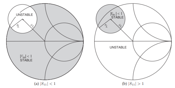
Figure \(\PageIndex{1}\): Output stability circles on the \(\Gamma_{L}\) plane. The shaded regions denote the values of \(\Gamma_{L}\) that will result in unconditional stability at the input indicated by \(|\Gamma_{\text{in}}| < 1\).

This defines a circle, called the output stability circle, in the \(\Gamma_{L}\) plane with center \(c_{L}\) and radius \(r_{L}\) (the development of this is given in Section 1.A.13) of [7]:

\[\label{eq:24}\text{center : }c_{L}=\frac{(S_{22}-\Delta S_{11}^{\ast})^{\ast}}{|S_{22}|^{2}-|\Delta |^{2}} \]

\[\label{eq:25}\text{radius : }r_{L}=\left|\frac{S_{12}S_{21}}{|S_{22}|^{2}-|\Delta |^{2}}\right| \]

This circle is plotted on a Smith chart in Figure \(\PageIndex{1}\) for the two conditions \(|S_{11}| < 1\) and \(|S_{11}| > 1\). When \(|S_{11}| < 1\) the shaded region in Figure \(\PageIndex{1}\)(a) indicates unconditional stability. That is, as long as \(\Gamma_{L}\) is chosen to lie in the shaded region, the input reflection coefficient, \(\Gamma_{\text{in}}\), will be less than one. It does not matter what the source impedance is, as long as it is passive there will not be oscillation due to multiple reflections between the input of the amplifier and the source.

Similarly an input stability circle can be defined for \(\Gamma_{S}\), where

\[\label{eq:26}\text{center : }c_{S}=\frac{(S_{11}-\Delta S_{22}^{\ast})^{\ast}}{|S_{11}|^{2}-|\Delta |^{2}} \]

\[\label{eq:27}\text{radius : }r_{S}=\left|\frac{S_{12}S_{21}}{|S_{11}|^{2}-|\Delta |^{2}}\right| \]

The interpretation of the input stability circles, shown in Figure \(\PageIndex{2}\), is similar to that for the output stability circles.

The stability criterion provided by the input and output stability circles is very conservative. For example, the input stability circle (for \(\Gamma_{S}\)) indicates the value of \(\Gamma_{S}\) that will ensure stability no matter what passive load is presented. Thus the stability circles here are called unconditional stability circles. However, an amplifier can be stable for loads (or source impedances) other than those that ensure unconditional stability. The use of stability circles provides a good first pass in design of the matching networks between the actual source and load and the amplifier. The stability circles will change with frequency, and so ensuring stability requires a broad frequency view. This is considered in the linear amplifier design case study in Section 2.9.

Shading is commonly used in publications to indicate the stable and

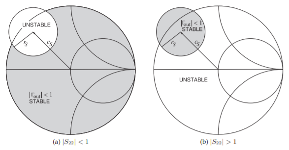
Figure \(\PageIndex{2}\): Input stability circles on the \(\Gamma_{S}\) plane. The shaded regions denote the values of \(\Gamma_{S}\) that will result in unconditional stability at the output indicated by \(|\Gamma_{\text{out}}| < 1\).

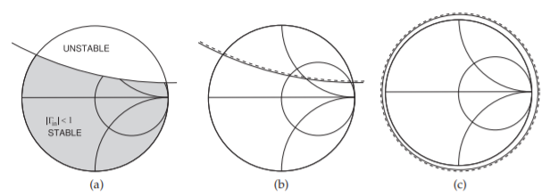
Figure \(\PageIndex{3}\): Stability circles: (a) using the absence of shading to indicate the potentially unstable region; (b) using a dashed line to indicate the same potentially unstable region; and (c) stability circle of an unconditionally stable (different) two-port.

potentially unstable regions on a Smith chart. An alternative commonly used by RF and microwave computer-aided design programs is to use a dashed line to indicate the side of the stability circle that is potentially unstable (see Figure \(\PageIndex{3}\)). Figure \(\PageIndex{3}\)(a) uses shading to indicate the potentially unstable region of the Smith chart while the stability circle in Figure \(\PageIndex{3}\)(b) indicates the potentially unstable region using a dashed line. The stability circle in Figure \(\PageIndex{3}\)(c) identifies a two-port that is stable for all passive terminations.

If an amplifier is unconditionally stable, amplifier design is considerably simplified. Matching network design then needs to be concerned about the impact of matching networks on stability. Detailed stability analyses are presented in [11] and [12]. Note that an amplifier can be stable even if it

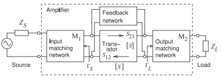
Figure \(\PageIndex{4}\): General amplifier configuration.

is not unconditionally stable.

2.6.3 Rollet's Stability Criterion — \(k\)-factor

Note

Rollet rhymes with wallet.

The \(k\)-factor method, also known as Rollet’s stability criterion [3, 4] is the most commonly used stability metric. It is based on the input and output reflection coefficients of an active device. The most general amplifier is depicted in Figure \(\PageIndex{4}\). Here the active device has scattering parameters

\[\label{eq:28}\mathbf{S}=[S]=\left[\begin{array}{cc}{S_{11}}&{S_{12}}\\{S_{21}}&{S_{22}}\end{array}\right] \]

and, as it will be used a lot, define the determinant \(\Delta = S_{11}S_{22} − S_{12}S_{21}\). The overall amplifier has scattering parameters \(\mathbf{S}′\). \(\Gamma_{S}\) is the generator reflection coefficient and \(\Gamma_{L}\) is the reflection coefficient of the load. For unconditional stability, \(|S'_{11}| < 1\) and \(|S'_{22}| < 1\). If \(|S'_{11}| > 1\) or \(|S'_{22}| > 1\), then there is a negative resistance and oscillation could possibly occur. Unconditional stability is defined as when \(|S'_{11}| < 1\) for all passive loads \(\Gamma_{L}\) (i.e., \(|\Gamma_{L}|\leq 1 )\) and \(|S'_{22}| < 1\) for all passive source impedances \(\Gamma_{S}\) (i.e., \(|\Gamma_{S}|\leq 1 )\). These inequalities are the same as saying the real part of the input and output impedances of the amplifier are positive resistances. These requirements also describe the unit circle on a Smith chart. Beginning with these definitions and ignoring the feedback network, a stability factor, \(k\), can be defined as

\[\label{eq:29}k=\left(\frac{1-|S_{11}|^{2}-|S_{22}|^{2}+|\Delta|^{2}}{2|S_{12}|\: |S_{21}|}\right) \]

where \(k > 1\) is required (but not sufficient) for unconditional stability. This is the Rollet stability condition. What is done here is rolling two unconditional stability requirements (on \(|S′_{11}|\) and \(|S′_{22}|\)) into one. If \(k\leq 1\), the amplifier may not be unstable, but extra care is required when a load is presented to the amplifier. If \(k > 1\), the design is relatively straightforward, but if \(k\) is near \(1\) or \(k\leq 1\), design will be troublesome. The closer design is to the limits of operation of a device, the more likely \(k\) will be near or less than \(1\). For example, the limit could be the maximum stable gain at the intended frequency of operation.

It has been shown that unconditional stability is assured if

\[\label{eq:30}k=\left(\frac{1-|S_{11}|^{2}-|S_{22}|^{2}+|\Delta |^{2}}{2|S_{12}|\: |S_{21}|}\right)>1 \]

Freq. \((\text{GHz}\))	\(k>1\)	\(|\Delta |<1\)	\(C_{L}\)	\(R_{L}\)	\(C_{S}\)	\(R_{S}\)
\(0.5\)	1\)">\(0.15178\)	\(0.62757\)	\(1.0388 + \jmath13.5176\)	\(13.370\)	\(0.92820 + \jmath0.50682\)	\(0.22434\)
\(1\)	1\)">\(0.24895\)	\(0.58720\)	\(0.78679 + \jmath7.26968\)	\(6.9988\)	\(0.69258 + \jmath0.96669\)	\(0.44107\)
\(2\)	1\)">\(0.46535\)	\(0.46821\)	\(0.73554 + \jmath3.96784\)	\(3.4718\)	\(−0.087892 + \jmath1.481129\)	\(0.72546\)
\(3\)	1\)">\(0.67865\)	\(0.37045\)	\(0.63608 + \jmath3.17780\)	\(2.4779\)	\(−0.86485 + \jmath1.46382\)	\(0.85475\)
\(4\)	1\)">\(0.91943\)	\(0.29706\)	\(0.52381 + \jmath2.82057\)	\(1.9223\)	\(−1.4232 + \jmath1.2217\)	\(0.91458\)
\(5\)	1\)">\(1.0838\)	\(0.24365\)	\(0.32018 + \jmath2.76164\)	\(1.7276\)	\(−1.90410 + \jmath0.77291\)	\(1.0132\)
\(6\)	1\)">\(1.1839\)	\(0.18765\)	\(0.065264 + \jmath2.679153\)	\(1.5700\)	\(−2.182123 + \jmath0.024217\)	\(1.0885\)
\(7\)	1\)">\(1.2846\)	\(0.14113\)	\(−0.39857 + \jmath2.97836\)	\(1.8266\)	\(−2.06262 − \jmath0.85258\)	\(1.0885\)
\(8\)	1\)">\(1.5225\)	\(0.092502\)	\(−0.91418 + \jmath3.21866\)	\(2.0150\)	\(−1.5996 − \jmath1.4914\)	\(0.94750\)
\(9\)	1\)">\(1.6448\)	\(0.056060\)	\(−1.2526 + \jmath3.0479\)	\(1.8998\)	\(−1.1418 − \jmath1.8922\)	\(0.92223\)
\(10\)	1\)">\(1.3151\)	\(0.072750\)	\(−1.7681 + \jmath2.6944\)	\(2.0189\)	\(−0.54178 − \jmath2.13439\)	\(1.0468\)
\(11\)	1\)">\(1.1043\)	\(0.11703\)	\(−2.6666 + \jmath2.4074\)	\(2.5186\)	\(0.24025 − \jmath2.02042\)	\(0.98357\)
\(12\)	1\)">\(0.98784\)	\(0.16159\)	\(−4.4423 + \jmath2.2978\)	\(4.0111\)	\(0.73109 − \jmath1.58120\)	\(0.74724\)
\(13\)	1\)">\(0.92131\)	\(0.18991\)	\(−5.9502 + \jmath1.0596\)	\(5.1100\)	\(0.96118 − \jmath1.24308\)	\(0.60117\)
\(14\)	1\)">\(0.84098\)	\(0.21905\)	\(−5.95467 − \jmath0.75389\)	\(5.1368\)	\(1.10689 − \jmath0.97667\)	\(0.53246\)
\(15\)	1\)">\(0.69555\)	\(0.24320\)	\(−6.0313 − \jmath1.9645\)	\(5.6068\)	\(1.20251 − \jmath0.58617\)	\(0.43291\)
\(16\)	1\)">\(0.63420\)	\(0.27993\)	\(−5.7310 − \jmath3.8333\)	\(6.2171\)	\(1.26271 − \jmath0.23704\)	\(0.39187\)
\(17\)	1\)">\(0.68792\)	\(0.32454\)	\(−3.5163 − \jmath5.6496\)	\(5.9268\)	\(1.257206 + \jmath0.087208\)	\(0.34232\)
\(18\)	1\)">\(0.72764\)	\(0.36197\)	\(−1.1258 − \jmath5.5386\)	\(4.8824\)	\(1.17955 + \jmath0.29932\)	\(0.27755\)
\(19\)	1\)">\(0.89194\)	\(0.35755\)	\(0.72551 − \jmath2.82689\)	\(1.9913\)	\(1.20751 + \jmath0.32462\)	\(0.27383\)
\(20\)	1\)">\(0.97085\)	\(0.32318\)	\(1.1030 − \jmath2.0753\)	\(1.3671\)	\(1.19540 + \jmath0.46897\)	\(0.29068\)
\(21\)	1\)">\(0.97475\)	\(0.28626\)	\(1.3859 − \jmath1.8451\)	\(1.3221\)	\(0.94075 + \jmath0.85514\)	\(0.27681\)
\(22\)	1\)">\(1.1014\)	\(0.28501\)	\(2.1696 − \jmath1.1961\)	\(1.4187\)	\(0.66834 + \jmath1.07377\)	\(0.24499\)
\(23\)	1\)">\(1.3123\)	\(0.29397\)	\(2.35683 − \jmath0.15064\)	\(1.1976\)	\(0.51539 + \jmath1.17421\)	\(0.22605\)
\(24\)	1\)">\(1.4714\)	\(0.28083\)	\(2.23754 + \jmath0.46967\)	\(1.0569\)	\(0.28045 + \jmath1.30061\)	\(0.24185\)
\(25\)	1\)">\(1.4273\)	\(0.22850\)	\(2.2473 + \jmath1.2506\)	\(1.3389\)	\(0.079906 + \jmath1.412442\)	\(0.31586\)
\(26\)	1\)">\(1.5308\)	\(0.17235\)	\(2.6309 + \jmath3.0590\)	\(2.6671\)	\(−0.45588 + \jmath1.43292\)	\(0.36774\)

Table \(\PageIndex{1}\): Rollet’s stability factor, \(k\)-factor, \(|\Delta |\), and stability circle parameters of the pHEMT transistor (in Table 2.3.1). For the active device to be unconditionally stable two conditions must be met: \(k > 1\) and \(|\Delta | < 1\). Frequencies at which the device is unconditionally stable (\(5–11\) and \(22–26\text{ GHz}\)) are in bold.

combined with any one of the following auxiliary conditions [13, 14, 15, 16, 17, 18, 19]:

\[\begin{align}\label{eq:31} B_{1}&=1+|S_{11}|^{2}-|S_{22}|^{2}-|\Delta |^{2}>0 \\ \label{eq:32}B_{2}&=1-|S_{11}|^{2}+|S_{22}|^{2}-|\Delta |^{2}>0 \\ \label{eq:33} |\Delta |&=|S_{11}S_{22}-S_{12}S_{21}|<1 \\ \label{eq:34}C_{1}&=1-|S_{11}|^{2}-|S_{12}S_{21}|>0 \\ \label{eq:35}C_{2}&=1-|S_{22}|^{2}-|S_{12}S_{21}|>0\end{align} \]

The conditions in Equations \(\eqref{eq:31}\)–\(\eqref{eq:35}\) are not independent, and it can be shown that one implies the others if \(k > 1\) [13].

Rollet’s stability criteria, \(k\) and \(|\Delta |\), are tabulated in Table \(\PageIndex{1}\) for the pHEMT described in Table 2.3.1. The device is unconditionally stable at the frequencies \(5–11\text{ GHz}\) and \(22–26\text{ GHz}\). It is seen that the device could be potentially unstable at frequencies below \(5\text{ GHz}\) and from \(12\) to \(21\text{ GHz}\). At these frequencies stability circles need to be used in designing matching networks.

Freq \((\text{GHz})\)	\(\mu >1\)	\(B_{1}>0\)	\(B_{2}>0\)	\(|\Delta |<1\)	\(C_{1}>0\)	\(C_{2}>0\)
\(0.5\)	1\)">\(0.18785\)	0\)">\(1.1555\)	0\)">\(0.056799\)	\(0.62757\)	0\)">\(−0.077921\)	0\)">\(0.47143\)
\(1\)	1\)">\(0.31338\)	0\)">\(1.1338\)	0\)">\(0.17657\)	\(0.58720\)	0\)">\(−0.080934\)	0\)">\(0.39770\)
\(2\)	1\)">\(0.56362\)	0\)">\(1.1086\)	0\)">\(0.45297\)	\(0.46821\)	0\)">\(0.065756\)	0\)">\(0.39356\)
\(3\)	1\)">\(0.76297\)	0\)">\(1.0884\)	0\)">\(0.63717\)	\(0.37045\)	0\)">\(0.22398\)	0\)">\(0.44958\)
\(4\)	1\)">\(0.94651\)	0\)">\(1.0631\)	0\)">\(0.76039\)	\(0.29706\)	0\)">\(0.35892\)	0\)">\(0.51029\)
\(5\)	1\)">\(1.0526\)	0\)">\(1.0434\)	0\)">\(0.83782\)	\(0.24365\)	0\)">\(0.44002\)	0\)">\(0.54284\)
\(6\)	1\)">\(1.1100\)	0\)">\(1.0341\)	0\)">\(0.89551\)	\(0.18765\)	0\)">\(0.49297\)	0\)">\(0.56225\)
\(7\)	1\)">\(1.1783\)	0\)">\(1.0703\)	0\)">\(0.88992\)	\(0.14113\)	0\)">\(0.51407\)	0\)">\(0.60424\)
\(8\)	1\)">\(1.3310\)	0\)">\(1.1120\)	0\)">\(0.87085\)	\(0.092502\)	0\)">\(0.54812\)	0\)">\(0.66871\)
\(9\)	1\)">\(1.3954\)	0\)">\(1.1104\)	0\)">\(0.88335\)	\(0.056060\)	0\)">\(0.57284\)	0\)">\(0.68634\)
\(10\)	1\)">\(1.2039\)	0\)">\(1.1068\)	0\)">\(0.88259\)	\(0.072750\)	0\)">\(0.51811\)	0\)">\(0.63023\)
\(11\)	1\)">\(1.0739\)	0\)">\(1.1550\)	0\)">\(0.81758\)	\(0.11703\)	0\)">\(0.43720\)	0\)">\(0.60592\)
\(12\)	1\)">\(0.99026\)	0\)">\(1.2715\)	0\)">\(0.67626\)	\(0.16159\)	0\)">\(0.33481\)	0\)">\(0.63244\)
\(13\)	1\)">\(0.93383\)	0\)">\(1.3461\)	0\)">\(0.58173\)	\(0.18991\)	0\)">\(0.27037\)	0\)">\(0.65257\)
\(14\)	1\)">\(0.86542\)	0\)">\(1.3788\)	0\)">\(0.52518\)	\(0.21905\)	0\)">\(0.22227\)	0\)">\(0.64910\)
\(15\)	1\)">\(0.73637\)	0\)">\(1.4578\)	0\)">\(0.42389\)	\(0.24320\)	0\)">\(0.13811\)	0\)">\(0.65507\)
\(16\)	1\)">\(0.67769\)	0\)">\(1.4752\)	0\)">\(0.36811\)	\(0.27993\)	0\)">\(0.099372\)	0\)">\(0.65290\)
\(17\)	1\)">\(0.72762\)	0\)">\(1.4461\)	0\)">\(0.34324\)	\(0.32454\)	0\)">\(0.10910\)	0\)">\(0.66053\)
\(18\)	1\)">\(0.76942\)	0\)">\(1.4300\)	0\)">\(0.30791\)	\(0.36197\)	0\)">\(0.10899\)	0\)">\(0.67006\)
\(19\)	1\)">\(0.92718\)	0\)">\(1.3348\)	0\)">\(0.40953\)	\(0.35755\)	0\)">\(0.18890\)	0\)">\(0.65152\)
\(20\)	1\)">\(0.98311\)	0\)">\(1.2924\)	0\)">\(0.49876\)	\(0.32318\)	0\)">\(0.24511\)	0\)">\(0.64191\)
\(21\)	1\)">\(0.98558\)	0\)">\(1.3331\)	0\)">\(0.50306\)	\(0.28626\)	0\)">\(0.24786\)	0\)">\(0.66286\)
\(22\)	1\)">\(1.0587\)	0\)">\(1.3627\)	0\)">\(0.47486\)	\(0.28501\)	0\)">\(0.25075\)	0\)">\(0.69466\)
\(23\)	1\)">\(1.1641\)	0\)">\(1.3295\)	0\)">\(0.49769\)	\(0.29397\)	0\)">\(0.28504\)	0\)">\(0.70093\)
\(24\)	1\)">\(1.2294\)	0\)">\(1.2872\)	0\)">\(0.55509\)	\(0.28083\)	0\)">\(0.33166\)	0\)">\(0.69771\)
\(25\)	1\)">\(1.2330\)	0\)">\(1.2866\)	0\)">\(0.60899\)	\(0.22850\)	0\)">\(0.36433\)	0\)">\(0.70313\)
\(26\)	1\)">\(1.3676\)	0\)">\(1.3398\)	0\)">\(0.60077\)	\(0.17235\)	0\)">\(0.38405\)	0\)">\(0.75358\)

Table \(\PageIndex{2}\): Edwards– Sinsky stability parameters for the pHEMT transistor documented in Table 2.3.1. For stability, \(\mu > 1\). The frequencies at which the device is unconditionally stable are in bold. The device is unconditionally stable at the frequencies \(5–11\text{ GHz}\) and \(22–26\text{ GHz}\). The other columns refer to Equations \(\eqref{eq:31}\)–\(\eqref{eq:35}\) and are provided for completeness.

2.6.4 Edwards-Sinsky Stability Criterion — \(\mu\)-factor

Rollet’s stability criterion, Equations \(\eqref{eq:30}\)–\(\eqref{eq:35}\), ensures unconditional stability but it does not provide a relative measure of stability. That is, the \(k\) factor cannot be used to determine how close a particular design is to the edge of stability. There is no ability to compare the relative stability of different designs. Edwards and Sinsky [13] developed a test that can be used to compare the relative stability of different designs. This is called the \(\mu\)-factor stability criterion, with unconditional stability having

\[\label{eq:36}\mu=\frac{1-|S_{11}|^{2}}{|S_{22}-S_{11}^{\ast}\Delta |+|S_{21}S_{12}|}>1 \]

An important result is that a larger value of \(\mu\) indicates greater stability. The \(\mu\) factor is a single quantity that provides a sufficient and necessary condition for unconditional stability. That is, it does not matter what passive source and load are presented (i.e. if \(|\Gamma_{S}|\leq 1\) and \(|\Gamma_{L}|\leq 1\)) then the amplifier will be stable if \(\mu > 1\). This contrasts with Rollet’s stability criterion in which two conditions must be met.

Edwards–Sinsky stability parameters for the pHEMT transistor (documented in Table 2.3.1) are shown in Table \(\PageIndex{2}\). The unconditionally stable frequencies of operation are \(5–11\text{ GHz}\) and \(22–26\text{ GHz}\). These are the same unconditionally stable frequencies determined by using Rollet’s stability criterion (in Table \(\PageIndex{1}\)). The additional information available with the Edwards–

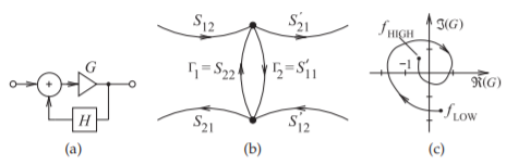
Figure \(\PageIndex{5}\): Nyquist stability analysis: (a) feedback amplifier; (b) a loop with reflection coefficients \(\Gamma_{1}\) and \(\Gamma_{2}\); and (c) a Nyquist stability plot of loop gain \(G = −\Gamma_{1}\Gamma_{2}\) (with \(H\) set to \(1\)).

Sinsky stability criterion is that \(\mu\) indicates the relative stability. In Table \(\PageIndex{2}\), the transistor is unconditionally stable in the \(5–11\text{ GHz}\) range, and in this range the device is most stable between \(8\) and \(10\text{ GHz}\). At the high end, above \(22\text{ GHz}\), the device is increasingly more stable. This can be expected to continue as the device capacitive parasitics short out the device. (The result of the low impedance of capacitors at high frequencies is that smaller RF voltages will be generated for the same drive level.) So this transistor will make a very good \(8–10\text{ GHz}\) amplifier provided that appropriate matching networks are chosen to ensure stability below \(5\text{ GHz}\) and above \(11\text{ GHz}\). Note, however, that the amplifier can be used up to about \(20\text{ GHz}\), but with extra care in design. Above \(20\text{ GHz}\) the maximum unilateral transducer gain is too small to be useful (see Table 2.3.3, where \(G_{TU\text{,max}}\) is tabulated for this transistor).

The Edwards–Sinsky stability factor, \(\mu\), is also called a geometric stability factor. It is the distance from the center of the Smith chart (i.e., the origin of the \(S\) parameter polar plot) to the nearest potentially unstable point on the input source plane. That is, it is the shortest distance from the origin to the input stability circle, where a negative \(\mu\) indicates that the stability circle encompasses the origin of the Smith chart.

Edwards and Sinsky also defined a dual parameter, \(\mu ′\) [13]:

\[\label{eq:37}\mu '=\frac{1-|S_{22}|^{2}}{|S_{11}-S_{22}^{\ast}\Delta |+|S_{21}S_{12}|} \]

This is the distance from the center of the Smith chart (i.e., the origin of the \(S\) parameter polar plot) to the nearest potentially unstable point on the output load plane. That is, it is the shortest distance from the origin to the output stability circle. If \(\mu > 1\) (indicating the possibility of two-port instability), then \(\mu′ > 1\) as well. Thus to determine whether or not a two-port is unconditionally stable, it is only necessary to consider one of them. Also, \(\mu\) and \(\mu ′\) are sometimes referred to as the input and output geometric stability factors respectively, and sometimes simply as \(\mu_{1}\) (MU1) and \(\mu_{2}\) (MU2), respectively. Calculating both \(\mu\) and \(\mu ′\) is useful, as this enables the relative stability at the input and the output to be examined. Table \(\PageIndex{3}\) lists \(\mu\) and \(\mu ′\) for the pHEMT transistor considered previously.

2.6.5 Nyquist Stability Criterion

The Nyquist stability criterion is the most complete way of analyzing stability. It is based on the analysis of the feedback system shown in Figure \(\PageIndex{5}\)(a) [20, 21, 22, 23]. The closed-loop transfer function is

\[\label{eq:38}T=\frac{G}{1+GH} \]

Freq. \((\text{GHz})\)	\(\mu\) (MU1) (input)	\(\mu '\) (MU2) (output)
\(0.5\)	\(0.18785\)	\(0.8332\)
\(1\)	\(0.31338\)	\(0.74811\)
\(2\)	\(0.56362\)	\(0.75828\)
\(3\)	\(0.76297\)	\(0.84547\)
\(4\)	\(0.94651\)	\(0.96112\)
\(5\)	\(1.05257\)	\(1.04174\)
\(6\)	\(1.10997\)	\(1.09373\)
\(7\)	\(1.17828\)	\(1.14339\)
\(8\)	\(1.33101\)	\(1.23947\)
\(9\)	\(1.39544\)	\(1.28779\)
\(10\)	\(1.20387\)	\(1.15528\)
\(11\)	\(1.07392\)	\(1.05108\)
\(12\)	\(0.99026\)	\(0.99479\)
\(13\)	\(0.93383\)	\(0.97018\)
\(14\)	\(0.86542\)	\(0.94371\)
\(15\)	\(0.73637\)	\(0.90486\)
\(16\)	\(0.67769\)	\(0.89289\)
\(17\)	\(0.72762\)	\(0.91790\)
\(18\)	\(0.76942\)	\(0.93939\)
\(19\)	\(0.92718\)	\(0.97655\)
\(20\)	\(0.98311\)	\(0.99342\)
\(21\)	\(0.98558\)	\(0.99451\)
\(22\)	\(1.05874\)	\(1.01979\)
\(23\)	\(1.16408\)	\(1.05629\)
\(24\)	\(1.22944\)	\(1.08865\)
\(25\)	\(1.23297\)	\(1.09884\)
\(26\)	\(1.36763\)	\(1.13596\)

Table \(\PageIndex{3}\): Input and output Edwards–Sinsky stability parameters for the pHEMT transistor documented in Table 2.3.1. For stability, \(\mu > 1\) and \(\mu ′ > 1\). The device is unconditionally stable at the frequencies \(5–11\text{ GHz}\) and \(22–26\text{ GHz}\).

The feedback system is unstable if the open-loop transfer function \(GH = −1\). Usually in stability analysis \(H\) is considered to be \(1\) so that the system is unstable if the open-loop transfer function \(G = −1\). Relating this to microwave circuits, every loop in a signal flow graph is considered. Generally it is sufficient to consider all possible loops containing one pair of nodes, as shown in Figure \(\PageIndex{5}\)(b). It would be best to select the pair of nodes at the input or output of an active device, as the active device is surely going to be involved in instability. There is of course a chance that the critical pair of nodes will be missed, which is more likely to happen in a multistage amplifier. In that situation several pairs of nodes should be considered individually. Returning to a single pair of nodes, as shown in Figure \(\PageIndex{5}\)(b), here the open-loop frequency-domain transfer function is

\[\label{eq:39}G=\Gamma_{1}\Gamma_{2} \]

The Nyquist stability criterion is that the system is unstable if the open-loop transfer function, \(G\), plotted on the complex plain encircles the \(−1\) point in a clockwise rotation with increasing frequency. The details behind this are provided in nearly every book on linear control systems (e.g. [20, 21, 22, 23]).

To ensure stability the Nyquist plot, as Figure \(\PageIndex{5}\)(c) is called, should be plotted for every loop in a system. However, experience is a good guide and only a few loops need to be considered in practice. There are also metrics such as the \(S\) probe parameter (sometimes called the \(G\) probe) used in microwave circuit simulators that provide a good estimate of whether the

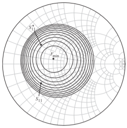
Figure \(\PageIndex{16}\): Noise figure circles at \(8\text{ GHz}\), plotted on the input Smith chart (i.e. on the \(\Gamma_{S}\) Smith chart) for the pHEMT transistor documented in Table 2.3.1. \(F_{\text{min}}\) is \(1.04\text{ dB}\) and the circles are in \(0.1\text{ dB}\) circles so that the outer circle is the locus of \(\Gamma_{S}\) that will produce a noise figure of \(2.04\text{ dB}\).

Nyquist plot will encircle the point [24]. The utility of this is that a twoport SPROBE or GPROBE element can be inserted into a circuit and used to provide a measure of Nyquist stability by considering the open-loop gain based on reflection coefficients looking from each port.

A similar technique to applying the Nyquist stability criterion is to create a Bode plot [25]. However, this is not easy to do with many microwave circuits and not often used.

2.6.6 Summary

This section presented criteria that can be used in determining the stability of transistor amplifiers and of active devices. Stability tests should be applied to the innermost two-port, specifically the active device, to provide an enhanced confidence in design. Two criteria in the forms of FOMs were presented for unconditional stability: the \(k\)-factor and \(\mu\)-factor. The \(k\)-factor, part of Rollet’s unconditional stability criterion, is a test of whether a device is unconditionally stable or not. It does not provide a relative measure of stability. The \(\mu\)-factor, derived by Edwards and Sinsky, is a factor that indicates the relative stability of a network. Stable amplifiers can be designed even if the amplifier is not unconditionally stable. Stability circles aid in the design of such amplifiers. Stability is an extensive topic and the reader is directed to in-depth stability analysis by Suarez and Quere [12] for further information.

Two graphical techniques were also presented. Stability circles can be used in design to enable graphically based trade-off of stability, noise, gain, and bandwidth information displayed on a Smith chart. It is surprising how well the trade-off can be made by a designer.