4.2: Simulation of Nonlinear Microwave Circuits

The circuit simulation tools used to model RF circuits are linear circuit simulators, transient circuit simulators (e.g., Spice), and nonlinear steady-state simulators. Transient circuit simulators can model large signals in RF circuits, but those available to RF designers cannot be used to model circuits requiring high dynamic range simulation or to model circuits with sharp frequency responses such as circuits with high-order filters. These simulators can be very slow, or perhaps impossibly slow, in modeling circuits with narrowband signals such as a digitally modulated carrier. When it is important to capture nonlinear and frequency-response effects precisely, nonlinear steady-state simulators are preferred. The two main types of nonlinear steady-state simulators available to designers are harmonic balance (HB) simulators [3, 4] and Spice-like transient simulators modified to efficiently find the response of a circuit to periodic excitation [5] (so-called periodic steady-state (PSS) analysis).

Nonlinear steady-state simulators exploit the narrowband nature of most radio systems and the circuit waveforms that are essentially steady-state, although not necessarily periodic. Such waveforms are called quasi-periodic waveforms. As an example of the waveforms to be determined, consider the

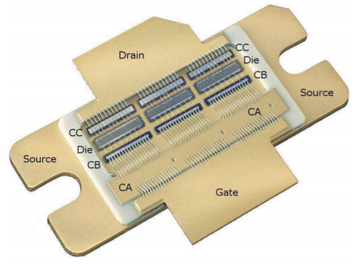
Figure \(\PageIndex{1}\): A \(2.1\text{ GHz}\) silicon LDMOS transistor. The gate and drain tabs are \(12.5\text{ mm}\) across. The three dies operate in parallel. The input matching network comprises a series inductance provided by bond wires, a shunt capacitor (Capacitor A, \(C_{A}\)), another series inductance from bond wires, and another shunt capacitor (\(C_{B}\)). The network is then connected to each gate finger of the transistor dies using short bond wires. The output matching network consists of a shunt capacitor (\(C_{C}\)) and series inductance. There are \(189\) bond wires. Used courtesy of Freescale Semiconductor Inc. Also see [1].

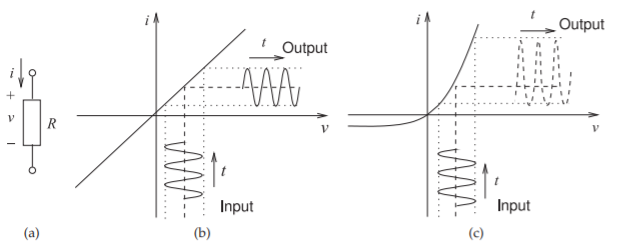
Figure \(\PageIndex{2}\): Current responses of a resistor: (a) resistor with passive convention defining voltage and current; (b) \(i-v\) characteristic of a linear resistor; and (c) \(i-v\) characteristic of a diode (a nonlinear resistor).

responses, shown in Figure \(\PageIndex{2}\), of linear and nonlinear resistors to an applied sinusoidal voltage.

Figure \(\PageIndex{2}\)(b) shows the \(i-v\) characteristic of a linear resistor. With an applied sinusoidal voltage, the output current waveform of the linear resistor is also a sinusoid. If the applied voltage signal is a sum of sinusoids, then the output current is also a sum of sinusoids. The component of output current at each frequency only depends on the applied voltage component at that frequency. With a nonlinear resistor having the \(i-v\) characteristic in Figure \(\PageIndex{2}\)(c), a large applied sinusoidal signal results in an output that is distorted and is a steady-state signal that has harmonics of the original signal. If the applied signal is the sum of two sinusoids of frequencies \(f_{1}\) and \(f_{2}\), then the output will be a steady-state signal with components having frequencies \(mf_{1} + nf_{2}\), where \(m\) and \(n\) are integers. The key feature here is that if a steady-state signal, a sum of sinusoids, is applied to a nonlinear circuit, then the output will also be a steady-state signal, a sum of sinusoids, but now each frequency component at the output is affected by every frequency component of the input signal. However, the simulation problem simplifies to finding the amplitudes and phases of the sinusoidal components rather than trying to determine the output waveform at a very large number of time points as done in a transient simulator. This is the basis of nonlinear steady-state simulation. In a narrowband radio, signals are very close to being sinusoidal with very slowly varying amplitude and phase [6].

4.2.1 Harmonic Balance Analysis of RF Circuits

With the harmonic balance method, the steady-state response of a nonlinear circuit is assumed to be a sum of sinusoids [3, 4]. This assumed form of the solution then allows simplification of the circuit equations, and simulation is used to determine the unknown coefficients: the magnitudes and phases of the sinusoids.

A harmonic-balance simulator can be many orders of magnitude more

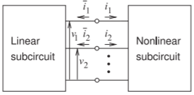
Figure \(\PageIndex{3}\): Analysis of a nonlinear circuit by the harmonic balance method partitions the circuit into linear and nonlinear subcircuits.

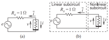
Figure \(\PageIndex{4}\): Example harmonic balance circuit: (a) circuit with nonlinear resistor; and (b) partitioned circuit. \(e(t) = E \cos(\omega y)\).

efficient than a time-domain simulator, and lends itself well to analysis of narrowband circuits and to optimization. Another major advantage of the harmonic balance method is that linear circuits can be of practically any size, with no significant increase in overall simulation time.

4.2.2 Example: Harmonic Balance Analysis of a Simple Circuit

Internally a harmonic balance simulator partitions a circuit into two subcircuits, as shown in Figure \(\PageIndex{3}\). During analysis, the set of frequencies being considered is fixed and the linear block need only be calculated initially, and its admittance parameters stored and reused at every stage of the analysis. Newton’s method (or similar iterative derivative-based minimization method) is used with harmonic balance to solve for the state of the circuit, that is, the amplitudes and phases of the voltage phasors at the interface.

As an example, consider the circuit in Figure \(\PageIndex{4}\)(a) where the nonlinear resistor is described by

\[\label{eq:1}i(t)=v(t)+[v(t)]^{2} \]

The first step in analysis partitions the circuit into linear and nonlinear subcircuits, as shown in Figure \(\PageIndex{4}\)(b). Harmonic balance simulation minimizes the frequency domain Kirchoff’s current law error at the linear circuit-nonlinear circuit interface. Next the number of sinusoids (or tones) to be considered must be chosen. The choice in this example is to consider only the DC, fundamental at radian frequency \(\omega\), and second-harmonic tones. Then the voltage at the interface is

\[\label{eq:2}v(t)=V_{0}+V_{1}\cos(\omega t)+V_{2}\cos(2\omega t) \]

Phase has been dropped, as this is a resistive circuit and all currents and voltages will have the same phase, nominally zero. Thus the unknowns are the amplitudes \(V_{0},\: V_{1},\) and \(V_{2}\). With values of \(V_{0},\: V_{1},\) and \(V_{2}\) assumed (and updated through iteration), the current flowing into the linear subcircuit can be calculated using the nodal admittance matrix of the linear subcircuit yielding

\[\label{eq:3}\overline{i}(t)=\overline{I}_{0}+\overline{I}_{1}\cos(\omega t)+\overline{I}_{2}\cos(2\omega t) \]

Similarly the nonlinear model of the element in the nonlinear subcircuit can be used to calculate the nonlinear currents:

\[\label{eq:4}i(t)=I_{0}+I_{1}\cos(\omega t)+I_{2}\cos(2\omega t) \]

The linear subcircuit, shown in Figure \(\PageIndex{4}\)(a), and the nonlinear subcircuit described by the quadratic model in Equation \(\eqref{eq:1}\) result in the following circuit equations:

\[\label{eq:5}\begin{array}{lll}{I_{0}=V_{0}+\frac{1}{2}V_{2}^{2}}&{I_{1}=V_{1}}&{I_{2}=\frac{1}{2}V_{1}^{2}} \\ {\overline{I}_{0}=V_{0}}&{\overline{I}_{1}=V_{1}-E}&{\text{and }\overline{I}_{2}=V_{2}}\end{array} \]

Since only the DC, fundamental, and second-harmonic components are being considered, the KCL error, \(F\), is

\[\label{eq:6}F=|f_{0}|+|f_{1}|+|f_{2}| \]

where the Kirchoff current error at DC, the fundamental, and the second harmonic are

\[\label{eq:7}f_{0}=I_{0}+\overline{I}_{0},\quad f_{1}=I_{1}+\overline{I}_{1},\quad\text{and}\quad f_{2}=I_{2}+\overline{I}_{2} \]

respectively. Thus \(F\) is minimized, or alternatively the zeros of each suberror, the \(f_{n}\)s, are found. The zeros can be found using a Newton–Raphson iterative technique to determine the voltages \((V_{0},\: V_{1},\) and \(V_{2})\) that yield the zeros of \(f_{0},\: f_{1},\) and \(f_{2}\). Thus the \((i + 1)\)th analysis iteration is

\[\label{eq:8} ^{^{^{^{i+1}}}}\left[\begin{array}{c}{V_{0}}\\{V_{1}}\\{V_{2}}\end{array}\right] =\:^{^{^{^{i}}}}\left[\begin{array}{c}{V_{0}}\\{V_{1}}\\{V_{2}}\end{array}\right]-\left[\mathbf{J}\left(^{^{^{^{i}}}}\left[\begin{array}{c}{V_{0}}\\{V_{1}}\\{V_{2}}\end{array}\right]\right)\right]^{-1}\times\left[\begin{array}{c}{f_{0}(^{i}[V_{0},\:V_{1},\:V_{2}]^{\text{T}})}\\{f_{1}(^{i}[V_{0},\:V_{1},\:V_{2}]^{\text{T}})}\\{f_{2}(^{i}[V_{0},\:V_{1},\:V_{2}]^{\text{T}})}\end{array}\right] \]

The Jacobian, \(\mathbf{J}\), is a matrix of derivatives of the \(f_{n}\)s with respect to the \(V_{n}\)s. Thus

\[\begin{align}&\mathbf{J}(^{i}[V_{0},\:V_{1},\:V_{2}]^{\text{T}})\nonumber \\ \label{eq:9}&= \left[\begin{array}{ccc}{\frac{\partial f_{0}(^{i}[V_{0},\:V_{1},\:V_{2}]^{\text{T}})}{\partial V_{0}}}&{\frac{\partial f_{0}(^{i}[V_{0},\:V_{1},\:V_{2}]^{\text{T}})}{\partial V_{1}}}&{\frac{\partial f_{0}(^{i}[V_{0},\:V_{1},\:V_{2}]^{\text{T}})}{\partial V_{2}}}\\{\frac{\partial f_{1}(^{i}[V_{0},\:V_{1},\:V_{2}]^{\text{T}})}{\partial V_{0}}}&{\frac{\partial f_{1}(^{i}[V_{0},\:V_{1},\:V_{2}]^{\text{T}})}{\partial V_{1}}}&{\frac{\partial f_{1}(^{i}[V_{0},\:V_{1},\:V_{2}]^{\text{T}})}{\partial V_{2}}}\\{ \frac{\partial f_{2}(^{i}[V_{0},\:V_{1},\:V_{2}]^{\text{T}})}{\partial V_{0}} }&{ \frac{\partial f_{2}(^{i}[V_{0},\:V_{1},\:V_{2}]^{\text{T}})}{\partial V_{1}} }&{ \frac{\partial f_{2}(^{i}[V_{0},\:V_{1},\:V_{2}]^{\text{T}})}{\partial V_{2}} }\end{array}\right]\end{align} \]

Now each element of the Jacobian is affected by both the linear and nonlinear subcircuits, so, for example,

\[\label{eq:10}\frac{\partial f_{2}(^{i}[V_{0},\:V_{1},\:V_{2}]^{\text{T}})}{\partial V_{1}}=\frac{\partial I_{2}(^{i}[V_{0},\:V_{1},\:V_{2}]^{\text{T}})}{\partial V_{1}}+\frac{\partial\overline{I}_{2}(^{i}V_{2})}{\partial V_{1}} \]

Since the linear current \(\overline{I}_{2}\) is dependent only on \(V_{2}\) (see Equation \(\eqref{eq:5}\),

\[\label{eq:11}\frac{\partial\overline{I}_{2}(^{i}V_{2})}{\partial V_{1}}=0 \]

and following trigonometric expansion of Equation \(\eqref{eq:1}\),

\[\label{eq:12}\frac{\partial I_{2}(^{i}[V_{0},\:V_{1},\:V_{2}]^{\text{T}})}{\partial V_{1}}=\frac{\partial}{\partial V_{1}}(\frac{1}{2}\:^{i}V_{1}^{2})=^{i}V_{1} \]

Similarly

\[\label{eq:13}\left.\begin{array}{ll}{\frac{\partial f_{0}(^{i}[V_{0},\:V_{1},\:V_{2}]^{\text{T}})}{\partial V_{0}}=1+2^{i}V_{0}+1}&{\frac{\partial f_{0}(^{i}[V_{0},\:V_{1},\:V_{2}]^{\text{T}})}{\partial V_{1}}=\:^{i}V_{1}}\\{ \frac{\partial f_{0}(^{i}[V_{0},\:V_{1},\:V_{2}]^{\text{T}})}{\partial V_{2}}= \:^{i}V_{2}}&{ \frac{\partial f_{1}(^{i}[V_{0},\:V_{1},\:V_{2}]^{\text{T}})}{\partial V_{0}}= 2^{i}V_{1}}\\{ \frac{\partial f_{1}(^{i}[V_{0},\:V_{1},\:V_{2}]^{\text{T}})}{\partial V_{1}}=1+2^{i}V_{0}+\:^{i}V_{2}+1 }&{ \frac{\partial f_{1}(^{i}[V_{0},\:V_{1},\:V_{2}]^{\text{T}})}{\partial V_{2}}=\:^{i}V_{1} }\\{ \frac{\partial f_{2}(^{i}[V_{0},\:V_{1},\:V_{2}]^{\text{T}})}{\partial V_{0}}=2^{i}V_{2} }&{ \frac{\partial f_{2}(^{i}[V_{0},\:V_{1},\:V_{2}]^{\text{T}})}{\partial V_{1}}= \:^{i}V_{1}}\\{ \frac{\partial f_{2}(^{i}[V_{0},\:V_{1},\:V_{2}]^{\text{T}})}{\partial V_{2}}= 2^{i}V_{0}+2}&{}\end{array}\right\} \]

Thus the equations to be solved by the harmonic balance simulator are

\[\label{eq:14}\left.\begin{array}{lllll}{^{i}I_{0}=\:^{i}V_{0}+\:^{i}V_{0}^{2}+V_{1}^{2}/2+V_{2}^{2}/2}&{\quad}&{^{i}\overline{I}_{0}=\:^{i}V_{0}}&{\quad}&{f_{0}=\:^{i}I_{0}+\:^{i}\overline{I}_{0}}\\{^{i}I_{1}=\:^{i}V_{1}+2^{i}V_{0}\:^{i}V_{1}+\:^{i}V_{1}\:^{i}V_{2}}&{\quad}&{^{i}\overline{I}_{1}=\:^{i}V_{1}-E_{1}}&{\quad}&{f_{1}=\:^{i}I_{1}+\:^{i}\overline{I}_{1}}\\{^{i}I_{2}=\:^{i}V_{2}+2^{i}V_{0}\:^{i}V_{2}+\:^{i}V_{1}^{2}/2}&{\quad}&{^{i}\overline{I}_{2}=\:^{i}V_{2}}&{\quad}&{f_{2}=\:^{i}I_{2}+\:^{i}\overline{I}_{2}}\end{array}\right\} \]

This is solved iteratively using the Newton–Raphson algorithm described by Equation \(\eqref{eq:8}\) to provide an updated estimate of the voltages (\(\:^{(i+1)}V_{0}\), \(^{(i+1)}V_{1}\), and \(^{(i+1)}V_{2}\)). The output of a program implementing this algorithm is shown in Table \(\PageIndex{1}\). Note how quickly the iterations arrive at the steady-state solution. This quick convergence to a steady-state solution is typical of harmonic balance simulation of nonlinear RF circuits.

The harmonic balance approach to nonlinear circuit analysis can be extended to consider excitation by sums of nonharmonically related sinusoids, which, for example, enables distortion to be determined using a two-tone test.

Many nonlinear RF circuits can be solved with just a few harmonics considered and only a few iterations are required to obtain convergence. The harmonic balance analysis is many orders of magnitude faster than simulation using transient circuit simulation and the dynamic range of the simulation can exceed \(150\text{ dB}\) while a transient simulator is often limited to dynamic ranges of \(80\text{ dB}\) and often much less is achieved. Consider a cell phone that can have transmit signals of up to \(30\text{ dBm}\), yet receive signals as small as \(−100\text{ dBm}\). Circuit simulation of such a system requires that the simulator have a dynamic range \(20\text{ dB}\) greater than the \(130\text{ dB}\) dynamic range of the cellphone signals. This is easily met by harmonic balance simulators. However, there are limitations to the use of the harmonic balance method.

ITERATION 0
\(\begin{align}\overline{I}_{0}&=0\nonumber \\ V_{0}&=0 \nonumber \\ I_{0}&=0.5\nonumber\end{align}\)	\(\begin{align}\overline{I}_{1}&=0\nonumber \\ V_{1}&=0.5\nonumber \\ I_{1}&=1\nonumber\end{align}\)	\(\begin{align}\overline{I}_{2}&=0\nonumber \\ V_{2}&=0\nonumber \\ I_{2}&=0.5\nonumber\end{align}\)
ITERATION 1
\(\begin{align}\overline{I}_{0}&=0\nonumber \\ V_{0}&=−0.0769231 \nonumber \\ I_{0}&=0.125\nonumber\end{align}\)	\(\begin{align}\overline{I}_{1}&=-0.5\nonumber \\ V_{1}&=0.557692\nonumber \\ I_{1}&=0.5\nonumber\end{align}\)	\(\begin{align}\overline{I}_{2}&=0\nonumber \\ V_{2}&=−0.0769231\nonumber \\ I_{2}&=0.125\nonumber\end{align}\)
ITERATION 2
\(\begin{align}\overline{I}_{0}&=−0.0769231\nonumber \\ V_{0}&=−0.0892028 \nonumber \\ I_{0}&=0.087463\nonumber\end{align}\)	\(\begin{align}\overline{I}_{1}&=−0.442308\nonumber \\ V_{1}&=0.57747\nonumber \\ I_{1}&=0.428994\nonumber\end{align}\)	\(\begin{align}\overline{I}_{2}&=−0.0769231\nonumber \\ V_{2}&=−0.0912325\nonumber \\ I_{2}&=0.0904216\nonumber\end{align}\)
ITERATION 3
\(\begin{align}\overline{I}_{0}&=−0.0892028\nonumber \\ V_{0}&=−0.089835 \nonumber \\ I_{0}&=0.0896515\nonumber\end{align}\)	\(\begin{align}\overline{I}_{1}&=−0.42253\nonumber \\ V_{1}&=0.578574\nonumber \\ I_{1}&=0.421762\nonumber\end{align}\)	\(\begin{align}\overline{I}_{2}&=−0.0912325\nonumber \\ V_{2}&=−0.0919462\nonumber \\ I_{2}&=0.0917795\nonumber\end{align}\)
ITERATION 4
\(\begin{align}\overline{I}_{0}&=−0.089835\nonumber \\ V_{0}&=−0.0898368 \nonumber \\ I_{0}&=0.0898363\nonumber\end{align}\)	\(\begin{align}\overline{I}_{1}&=−0.421426\nonumber \\ V_{1}&=0.578577\nonumber \\ I_{1}&=0.421424\nonumber\end{align}\)	\(\begin{align}\overline{I}_{2}&=−0.0919462\nonumber \\ V_{2}&=−0.0919482\nonumber \\ I_{2}&=0.0919477\nonumber\end{align}\)
ITERATION 5
\(\begin{align}\overline{I}_{0}&=−0.0898368\nonumber \\ V_{0}&=−0.0898368 \nonumber \\ I_{0}&=0.0898368\nonumber\end{align}\)	\(\begin{align}\overline{I}_{1}&=−0.421423\nonumber \\ V_{1}&=0.578577\nonumber \\ I_{1}&=0.421423\nonumber\end{align}\)	\(\begin{align}\overline{I}_{2}&=−0.0919482\nonumber \\ V_{2}&=−0.0919482\nonumber \\ I_{2}&=0.0919482\nonumber\end{align}\)
ITERATION 6
\(\begin{align}\overline{I}_{0}&=−0.0898368\nonumber \\ V_{0}&=−0.0898368 \nonumber \\ I_{0}&=0.0898368\nonumber\end{align}\)	\(\begin{align}\overline{I}_{1}&=−0.421423\nonumber \\ V_{1}&=0.578577\nonumber \\ I_{1}&=0.421423\nonumber\end{align}\)	\(\begin{align}\overline{I}_{2}&=−0.0919482\nonumber \\ V_{2}&=−0.0919482\nonumber \\ I_{2}&=0.0919482\nonumber\end{align}\)
ITERATION 7
\(\begin{align}\overline{I}_{0}&=−0.0898368\nonumber \\ V_{0}&=−0.0898368 \nonumber \\ I_{0}&=0.0898368\nonumber\end{align}\)	\(\begin{align}\overline{I}_{1}&=−0.421423\nonumber \\ V_{1}&=0.578577\nonumber \\ I_{1}&=0.421423\nonumber\end{align}\)	\(\begin{align}\overline{I}_{2}&=−0.0919482\nonumber \\ V_{2}&=−0.0919482\nonumber \\ I_{2}&=0.0919482\nonumber\end{align}\)
stop

Table \(\PageIndex{1}\): Circuit quantities at each iteration in the harmonic balance analysis of the circuit in Figure \(\PageIndex{4}\)(a).

A major drawback is that harmonic balance does not work well with circuits containing large numbers of transistors, say a few tens of transistors. This is largely because the Jacobian becomes very large and analysis becomes unwieldy.

4.2.3 User's Guide to Using Harmonic Balance Analysis

Three major factors limit the accuracy of harmonic balance circuit simulation:

1. The number of tones included in the analysis. If the number of tones is too small, there will be truncation error. Truncation error arises because, theoretically, an infinite number of harmonics can be generated by the interaction of large signals with even simple nonlinear circuits. The error can be reduced, of course, by specifying additional frequency components.
2. The aliasing errors due to a finite transform spectrum. This error can be reduced by considering many tones. The aliasing error is a numerically introduced error. This sets an upper limit on resolution.
3. The final value of the harmonic balance error. The major limiting factor here is how closely the Jacobian describes the actual error function. Both the error function and the Jacobian have truncation error so ideally the Jacobian evaluation reflects the same truncation errors as the error function evaluation. In the end this comes down to the accuracy of the models. That is, whether the derivatives calculated in the model reflect the actual nonlinear relationship.

Naturally errors also arise due to the quality of the models of the active devices and of the linear circuit elements. Also, as the number of tones included in a harmonic balance analysis increases, the simulation time rapidly increases

4.2.4 Periodic Steady-State Simulation of RF Circuits

Periodic steady-state (PSS) analysis is used with a Spice simulator to establish the response of a circuit to a periodic excitation signal [5]. Typically there would be one large sinusoid, such as a local oscillator or a carrier signal. The idea is that the dynamic state of the circuit is established by a transient simulation with a single sinusoidal excitation. Then a linear (or perhaps quadratic) model of the dynamic circuit is used with smaller signals. If the excitation signal is large, then the circuit is a time-varying linear circuit as far as smaller signals are concerned.

The PSS technique uses what is called the shooting method in which the simulator guesses the initial values of voltages at all terminals, charges on all capacitors, and currents through all inductors (i.e., the state-variables of the circuit) [7, 8, 9, 10, 11, 12, 13]. Then the circuit is simulated using transient analysis for one period of the exciting waveform. The state variables after one period are compared to the assumed state variables at the beginning of the period. If there is a difference, then the initial guess is changed and the process repeated. Convergence is usually achieved after a few iterations. Then the Fourier components of the state variables are found and a time-varying circuit calculated. From this, a model akin to a conversion matrix describing the dynamic circuit is established. There are many similarities to harmonic balance, as the frequencies of all signals in the circuit must be specified by the user. An advantage of the PSS technique is that a conventional Spice simulator, and the all important transistor models, can be used.