4.4: Distortion and Digitally Modulated Signals

Digitally-modulated signals do not have constant envelopes so that the short-term peak power of the RF signal is higher than the average RF power. Efficient amplifiers must introduce minimal distortion and be efficient for peak signal levels as well as for the average signal level. There is a tradeoff between distortion and efficiency and various amplifier architectures have been developed to implement good trade-offs. These architectures will be introduced in a later section. This section introduces approaches for describing distortion.

4.4.1 PMEPR and Probability Density Function

Amplitude variations occur with most digital modulation schemes. For example, a QPSK signal consists of two digital data streams, equal in amplitude, modulated in quadrature onto a carrier signal. If the data streams are not filtered prior to modulation, then the resulting modulated carrier signal has a constant envelope with instantaneous transitions from one constellation point to another. However, the occupied bandwidth of this signal is quite large, as the spectrum is that of a pulse train, \(\sin(x)/x\), the \(\text{sinc}\) function. The first sidelobe of the \(\text{sinc}\) spectrum is only \(13\text{ dB}\) down from the carrier level and typically is in the middle of the adjacent channel. To reduce the bandwidth of the modulated signal, a low-pass filter is applied to each digital data stream to minimize the out-of-band spectrum of the modulated signal. This comes with a drawback: the filters cause a finite memory effect resulting in amplitude variations as the ringing energy from a previous data pulse adds to the current filtered data pulse. As well, the transitions from one constellation point to another are slow and the amplitude of the modulated carrier varies significantly during the transition.

Amplitude variations of the modulated signal are characterized by waveform statistics such as the PMEPR. A signal with a high PMEPR requires that the RF system have high linearity to handle both the average power requirements and the peak amplitude excursions without generating excessive out-of-band distortion. A simple design technique is to reduce the average output power of an amplifier to a level that is below the \(1\text{ dB}\)

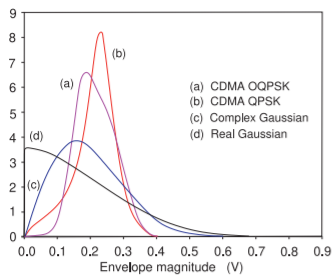
Figure \(\PageIndex{1}\): Amplitude PDF for CDMA and Gaussian modulated signals with the same power of \(0\text{ dBm}\). After [31].

Signal Modulation	PMEPR (dB)
CDMA OQPSK	\(5.4\)
CDMA QPSK	\(6.6\)
Real Gaussian	\(13.5\)
Complex Gaussian	\(11.8\)

Table \(\PageIndex{1}\): Peak-to-average ratios in decibels for OQPSK and QPSK used in CDMA compared to the PMEPRs of Gaussian signals.

gain compression power by the PMEPR, this is called amplifier back-off. However, it is possible for a signal with a high PMEPR to exhibit less nonlinear distortion than a signal with lower PMEPR [30]. The reason for this apparent inconsistency is because the signal peak may have a low probability of occurrence. Thus PMEPR by itself is an incomplete statistic for determining the linearity requirements of an amplifier.

The amplitude probability density function (APDF) is a more complete statistical description of the amplitude variations of a modulated signal. The APDF defines the maximum and minimum variation along with the relative probability of occurrence of amplitudes within the variation. The APDF is typically estimated from a histogram of envelope amplitudes, with a uniform bin size, by

\[\label{eq:1}f(A)=\frac{N}{\Delta A\times N_{c}} \]

where \(N\) is the number of counts in the bin having amplitude \(A\), \(\Delta A\) is the bin width (i.e., the range of amplitudes in the bin), and \(N_{c}\) is the total number of samples. The shape of the amplitude density determines the sensitivity of a particular signal to spectral regrowth due to nonlinear gain compression or expansion. This is a more precise determinant of distortion than the single PMEPR metric.

As an example, consider Figure \(\PageIndex{1}\) which shows the APDF of a CDMA signal using OQPSK modulation, of the same signal but now using QPSK modulation of a real Gaussian signal and of a complex Gaussian QPSK signal (with \(I\) and \(Q\) each having Gaussian distributions) where the average power of each signal is set to \(0\text{ dBm}\). Gaussian signals are of particular interest because their simple statistics lend them, and their interaction with nonlinear circuits, to quasi-analytic treatment [32]. The PMEPR of each signal is given in Table \(\PageIndex{1}\). From the shape of the APDF it is possible to estimate which signal will be more sensitive to nonlinear gain compression.

For example, even though QPSK has a higher PMEPR than OQPSK, the probability that the OQPSK envelope is near the peak is higher than for the QPSK signal. This is seen in Figure \(\PageIndex{1}\). It is not surprising then that the measured spectral regrowth of an OQPSK signal is higher than that for a QPSK signal. So PMEPR is only a rough guide to the distortion that is produced.

4.4.2 Design Guidelines

Generally an amplifier is not operated in saturation nor near the third-order intercept (TOI or IP3) point. An exception is with constant or near-constant envelope modulation schemes such as FM, GMSK, SOQPSK, FOQPSK, and SBPSK. With little variation in the amplitude of the RF signal, saturating amplifiers can be used with the near-constant envelope schemes. Also some advanced amplifier technologies can operate with nonlinear transistor loadlines and still have low distortion. For example, with some switching amplifiers produce little intermodulation distortion but a lot of harmonic distortion which is easily filtered out. With nonconstant envelope modulation schemes (i.e., the signal PMEPR is more than \(0\text{ dB}\)), the variation in the amplitude of the modulated RF carrier results in signal distortion and spectral regrowth (i.e., power will be transferred into neighboring communication channels). One general rule of design is to ensure that the peak of the RF pseudo-carrier is at or below the \(1\text{ dB}\) gain compression point. The amplifier is backed off by an amount approximately PMEPR below the \(1\text{ dB}\) gain compression point. Generally, however, third-order intermodulation is a much greater concern, as this relates more closely to the amount of power dumped into neighboring channels.

Modern communication schemes can require that the adjacent channel spectral regrowth be as much as \(80\text{ dB}\) below the power of the main channel. As a result, the signal must be backed off considerably from the IP3 point. The input or output power at IP3 (IIP3 or OIP3) is obtained from two-tone characterization and thus is a weakly accurate indicator of distortion with a digitally modulated signal. However, since it is a simple measurement to make and understand, it is widely used. Experience provides a rule of thumb for the backoff needed to ensure a maximum level of spectral regrowth for a particular modulation format and transistor technology [21].

Since the complexity of designing high-power and highly efficient amplifiers is considerable, it is necessary to use measurements following design to optimize the system for high efficiency while ensuring acceptable distortion. The most common measurement approach is to use loadpull, described in the next section. Design of the baseband circuit can also affect intermodulation distortion and spectral regrowth [33, 34, 35]. It is very important that the transistor ground be the system ground and that there be good heat-sinking so that the thermal circuit does not contribute to spectral regrowth through the variation of thermally dependent transistor parameters as the signal envelope varies (and thus the heat generated varies).

While IP3 and the \(1\text{ dB}\) compression point only refer to amplitude distortion, there will also be phase distortion. While amplitude distortion has no effect on constant amplitude signals, phase distortion does. Phase distortion affects the performance of constant envelope modulation schemes

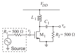
Figure \(\PageIndex{2}\): Class A inductively-biased MOSFET amplifier.

and the \(1\text{ dB}\) compression point and IP3 provide some indication of possible phase distortion. Although EVM and BER are much better metrics of distortion for all digital modulation schemes, these are difficult to use in guiding initial design of RF hardware.

Example \(\PageIndex{1}\): Intercept Point

The dynamic range derivations in Section 4.6 of [2] should be reviewed before working through this example.

The amplifier shown in Figure \(\PageIndex{2}\) is modeled, after expansion around the operating point, by a nonlinear transconductance with \(i_{DS} = a_{1}v_{GS} + a_{3}v_{GS}^{3}\) with \(a_{1} = 0.01\text{ A/V}\) and \(a_{3} = −0.1\text{ A/V}^{3}\). \(L_{1}\) is an RF choke and can be assumed to present an open circuit at the operating frequency. \(C_{1}\) is a biasing capacitor and can be treated as a short circuit at the operating frequency. \(R_{2}\) is the load resistance.

1. What is the small signal voltage gain of the amplifier?
2. If the input signal is a two-tone signal consisting of two equal-amplitude sinewaves at \(900\text{ MHz}\) and \(901\text{ MHz}\), what are the frequencies in the spectrum of \(v_{o}\)? Determine the output voltage across \(R_{2}\)?
3. If a single sinusoid of amplitude \(100\text{ mV}\) is applied to the gate of the MOSFET, what is the level of the fundamental tone at the output of the amplifier? What is the level of the third harmonic?
4. What is the input-referred third-order intercept point, IIP3, of the amplifier?
5. What is the output-referred third-order intercept point, OIP3, of the amplifier?

Solution

1. When the input signal \(v_{i}\) is small, \(i_{DS} = a_{1}v_{i}\), so the small signal output voltage is
   \[v_{o}=-i_{DS}R_{2}=-a_{1}R_{2}v_{i}\nonumber \]
   and the small signal voltage gain is
   \[A=\frac{v_{o}}{v_{i}}=-a_{1}R_{2}=-0.01\times 500=-5\nonumber \]
2. Eventually the symbolic amplitudes of the mixing terms will be required, so a trigonometric expansion is undertaken now. To minimize complexity, consider two cosinsoids, \(A \cos(x)\) and \(B \cos(y)\). So the input to the amplifier is
   \[v_{GS}=A\cos(x)+B\cos(y)\nonumber \]
   The output of the amplifier is
   \[\begin{align}v_{o}&=-i_{DS}R_{2}=-R_{2}(a_{1}v_{GS}+a_{3}V_{GS}^{3})\nonumber \\ &=-R_{2}\{a_{1}[A\cos(x)+B\cos(y)]+a_{3}[A\cos(x)+B\cos(y)]^{3}\}\nonumber \\ &=-R_{2}\{a_{1}[A\cos(x)+a_{1}B\cos(y)]+a_{3}[A\cos(x)+B\cos(y)]\:[A\cos(x)+B\cos(y)]^{2}\}\nonumber \\ &=-R_{2}\{a_{1}[A\cos(x)+a_{1}B\cos(y)]\nonumber \\ &\quad +a_{3}[A\cos(x)+B\cos(y)]\:[A^{2}\cos^{2}(x)+2AB\cos(x)\cos(y)+B^{2}\cos^{2}(y)]\}\nonumber \\ &=-R_{2}\{a_{1}A\cos(x)+a_{1}B\cos(y)\nonumber \\ &\quad +a_{3}[A\cos(x)+B\cos(y)]\nonumber \\ &\quad\times\frac{1}{2}[A^{2}+B^{2}+A^{2}\cos(2x)+B^{2}\cos(2y)+2AB\cos(x-y)+2AB\cos(x+y)]\}\nonumber \\ &=-R_{2}\{a_{1}[A\cos(x)+B\cos(y)]\nonumber \\ &\quad +a_{3}\frac{1}{2}[(A^{3}+AB^{2})\cos(x)+A^{3}\cos(x)\cos(2x)+AB^{2}\cos(x)\cos(2y)\nonumber \\ &\quad +2A^{2}B\cos(x)\cos(x-y)+2AB^{2}\cos(x)\cos(x+y)+(A^{2}B+B^{3})\cos(y)\nonumber \\ &\quad +B^{3}\cos(y)\cos(2y)+A^{2}B\cos(y)\cos(2x)+2AB^{2}\cos(y)\cos(x-y)\nonumber \\ &\quad +2AB^{2}\cos(y)\cos(x+y)]\}\nonumber \\ &=-R_{2}(a_{1}[A\cos(x)+a_{1}B\cos(y)]\nonumber \\ &\quad +a_{3}\frac{1}{2}\{(A^{3}+AB^{2})\cos(x)+\frac{1}{2}A^{3}[\cos(x)+\cos(3x)]\nonumber \\ &\quad +\frac{1}{2}AB^{2}[\cos(2y-x)+\cos(x+2y)]+A^{2}B[\cos(y)+\cos(2x-y)]\nonumber \\ &\quad +A^{2}B[\cos(y)+\cos(2x+y)]+(A^{2}B+B^{3})\cos(y)\nonumber \\ &\quad+\frac{1}{2}B^{3}[\cos(y)+\cos(3y)]+\frac{1}{2}A^{2}B[\cos(2x-y)+\cos(2x+y)]\nonumber \\ &\quad +AB^{2}[\cos(x)+\cos(2y-x)]+AB^{2}[\cos(x)+\cos(2y+x)]\})\nonumber \\ &=-R_{2}\{a_{1}A\cos(x)+a_{1}B\cos(y)+a_{3}\frac{1}{4}[(3A^{3}+6AB^{2})\cos(x)\nonumber \\ &\quad +(3B^{3}+6AB^{2})\cos(y)+B^{3}\cos(3y)+3A^{2}B\cos(2x-y)\nonumber \\ \label{eq:2}&\quad +3A^{2}B\cos(2x+y)+A^{3}\cos(3x)+3AB^{2}\cos(2y-x)+3AB^{2}\cos(2y+x)]\} \end{align} \]
   So with \(x\) representing \(900\text{ MHz}\) and \(y\) representing \(901\text{ MHz}\), the frequencies in the output spectrum are \(899,\: 900,\: 901,\) \(902,\: 2700,\: 2701,\) \(2702,\) and \(2703\text{ MHz}\).
3. From Equation \(\eqref{eq:2}\) and considering only one tone (i.e., \(B = 0\)), the output signal is
   \[\label{eq:3}v_{o}=-R_{2}\left[a_{1}A\cos(x)+\frac{3a_{3}A^{3}}{4}\cos(x)+\frac{a_{3}A^{3}}{4}\cos(x)\right] \]
   So the coefficient of the fundamental at the output is
   \[\label{eq:4}v_{o}=-R_{2}\left[a_{1}A\cos(x)+\frac{3a_{3}A^{3}}{2}\cos(x))\right] \]
   Here \(A = 100\text{ mV}\), so the
   \[\begin{align}\text{fundamental output }&=-(500\:\Omega)\cdot [(0.01\text{ A/V})\cdot (0.5\text{ V})+(-0.1\text{ A/V}^{3})\cdot (0.1\text{ V})^{3}]\nonumber \\ \label{eq:5}&=0.05-0.0125\text{ V}=0.0375\text{ V}=37.5\text{ mV} \\ \label{eq:6}\text{third harmonic output }&=\frac{a_{3}R_{2}}{4}v_{i}^{3}=(-500)\cdot (-0.1)\times (0.1)^{3}/4=0.0125\text{ V}\end{align} \]
4. To answer this, determine the level of the fundamental and IM3 outputs for small \(v_{GS}\) and for two input tones having the same amplitude, \(A = B = v_{GS}\). For a resistive nonlinearity, such as the transconductance here, the level of the lower and upper third-order intermods are the same. So, after examining Equation \(\eqref{eq:2}\), consider \(\cos(x)\) and \(\cos(2x − y)\). The fundamental (at \(\cos(x)\)) is
   \[v_{o}(900\text{ MHz})=-R_{2}a_{1}v_{i}\nonumber \]
   and the level of the lower third-order intermod at \((2x − y)\) is
   \[v_{o}(899\text{ MHz})=-R_{2}a_{3}\frac{3}{4}(v_{i})^{3}\nonumber \]
   IIP3 is the value of \(v_{i}\) when \(v_{o}(900\text{ MHz}) = v_{o}(899\text{ MHz})\), that is, when
   \[-R_{2}a_{1}v_{i}=-R_{2}a_{3}\frac{3}{4}(v_{i})^{3}\nonumber \]
   That is, when
   \[v_{i}=\sqrt{\left|\frac{4a_{1}}{3a_{3}}\right|}=\sqrt{\frac{4\cdot 0.01}{3\cdot 0.1}}=0.3651\text{ V}=365.1\text{ mV}\nonumber \]
   Thus
   \[A_{\text{IIP3}}=365.1\text{ mV}\nonumber \]
   Normally IIP3 is expressed in terms of power. Considering Figure \(\PageIndex{2}\), \(E = 2v_{i}\), and so the available input power is
   \[P_{\text{av}}=\frac{1}{2}\frac{v_{i}^{2}}{R_{1}}=\frac{v_{i}^{2}}{2R_{1}}\nonumber \]
   Thus
   \[\text{IIP3}=\frac{1}{2R_{1}}A_{\text{IIP3}}^{2}=\frac{0.3651^{2}}{2\cdot 500}=0.0001333\text{ W}=0.1333\text{ mw}=-0.875\text{ dBm}\nonumber \]
5. The voltage output-referred intercept point is
   \[A_{\text{OIP3}}=|A|\: A_{\text{IIP3}}=5\cdot 0.3651\text{ V}=1.8255\text{ V}\nonumber \]
   and
   \[\text{OIP3}=(\text{Power gain})\cdot\text{IIP3}=\frac{R_{1}}{R_{2}}A^{2}\cdot 0.1333\text{ mW}=3.333\text{ mW}=5.23\text{ dBm}\nonumber \]