4.8: Advanced Power Amplifier Architectures

A central challenge of power amplifier design is trading off power efficiency and distortion. Up to now discussion has focused on efficient design of single transistor amplifiers. In this section several architectures are described that enable the efficiency-distortion trade-off to go to a higher level. The three architectures discussed are the Doherty amplifier, the envelope tracking amplifier, the LITMUS amplifier, and the LINC amplifier.

4.8.1 Doherty Amplifier

A Doherty amplifier improves linearity and achieves high efficiency by using two amplifiers, one called a carrier amplifier and the other a peaking amplifier [45, 46, 51, 52, 53, 54, 55]. The basic Doherty amplifier configuration is shown in Figure \(\PageIndex{1}\)(a). Here the input signal is split and half is applied to the carrier amplifier, typically a low-distortion Class AB amplifier, which amplifies small signals. However, as the input signal increases this amplifier becomes nonlinear and saturates, as seen in Figure \(\PageIndex{1}\)(b). The other amplifier is typically a Class C amplifier and does not amplify small signals, but as the input becomes larger, the amplifier turns on. The Doherty amplifier has high linearity, as at high input powers the turn-on characteristic of the peaking amplifier complements the saturation of the carrier amplifier. The essential operation is that the input signal is split and half is shifted by \(90^{\circ}\). At the output this phase shift is matched by the \(90^{\circ}\) electrical length of the transmission line at the output of the carrier amplifier. This transmission line efficiently routes the output of the carrier amplifier to the load whether or not the peaking amplifier is turned on. When it is not turned on, the peaking amplifier presents an open circuit, but when it is on, it presents a Thevenin impedance \(Z_{0}\). Then, the output power of both the carrier and peaking amplifiers are efficiently combined.

A more complete circuit design of an HBT Doherty amplifier is shown in Figure \(\PageIndex{2}\). The \(90^{\circ}\) hybrid at the input splits the signals and introduces the required phase shift. Base biasing voltages of the HBT transistors (i.e. \(V_{bc}\) and \(V_{bp}\)) are adjusted so that the carrier amplifier will amplify small signals, but the peaking amplifier will have a Class C-like characteristic and only turn on for large signals.

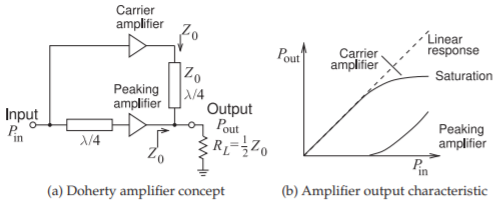
Figure \(\PageIndex{1}\): Doherty amplifier.

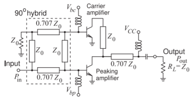
Figure \(\PageIndex{2}\): HBT Doherty amplifier with a \(90^{\circ}\) hybrid between \(P_{\text{in}}\) and the input of the transistors. All lines are \(\lambda /4\) (i.e. \(90^{\circ}\)) long.

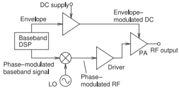
Figure \(\PageIndex{3}\): Khan transmitter using envelope elimination and restoration.

4.8.2 Envelope Tracking Amplifier

The concept of the envelope tracking amplifier was introduced with the Khan transmitter [56, 57, 58, 59]. This technique is also called the envelope-elimination and restoration (EER) technique. The original amplifier concept [56], but updated to use modern DSP capabilities, is shown in Figure \(\PageIndex{3}\). The DSP operates at baseband and produces the digitally modulated signal to be transmitted. The DSP separately produces an amplitude-varying envelope signal and a constant-envelope phase-modulated baseband signal. These are amplified separately. This is in contrast to the usual approach of producing a baseband signal, or even a low-power RF signal, which has the complete modulation with both phase and amplitude variations. The phase-modulated signal is amplified by a driver before it is input to an efficient power amplifier that always operates in a highly linear mode since the DC source to the PA is adjusted to match the envelope of the final signal. Thus the PA is always operating at peak efficiency. These amplifiers have excellent linearity over a broad frequency range.

4.8.3 LINC Amplifier

The linear amplification with nonlinear component (LINC) amplifier separates a digitally modulated signal into two constant envelope components [18, 60, 61, 62]. This amplifier is also known as an outphasing amplifier. Each of the components is efficiently amplified by individual amplifiers and then recombined. The amplifier concept is shown in Figure \(\PageIndex{4}\).

The LINC amplifier operates as follows. The digitally modulated RF input signal can be expressed as

\[\label{eq:1}s(t)=a(t)\cos[\omega t +\theta (t)] \]

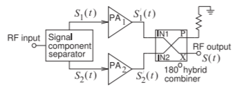
Figure \(\PageIndex{4}\): LINC amplifier.

In complex exponential form this becomes

\[\label{eq:2}s(t)=a(t)\text{e}^{\jmath\theta (t)} \]

where \(a(t)\) describes the amplitude modulation of the signal and \(\theta (t)\) describes the phase modulation of the signal. This signal is split by the signal component separator to create two components, \(S_{1}′(t)\) and \(S_{2}′(t)\), with the same constant amplitudes and with complementary time-varying phase modulation:

\[\begin{align}\label{eq:3}S_{1}(t)&=\frac{1}{2}[s(t)-e(t)]_{\text{I}}=\frac{1}{2}V_{m}\cos[\omega t+\theta (t)-\psi (t)] \\ \label{eq:4}S_{2}(t)&=\frac{1}{2}[s(t)+e(t)]_{\text{I}}=\frac{1}{2}V_{m}\cos[\omega t+\theta (t)+\psi (t)]\end{align} \]

where \(\psi (t) = \cos^{−1} [a(t)/V_{m}]\), the subscript \(\text{I}\) denotes the in-phase component and \(\frac{1}{2}V_{m}\) is the magnitude of the voltage signal applied to each of the PAs. The \(e(t)\) term is called the quadrature signal and

\[\label{eq:5}e(t)=\jmath s(t)\sqrt{\frac{V_{m}^{2}}{a^{2}(t)}-1} \]

\(S_{1}(t)\) and \(S_{2}(t)\) are efficiently amplified separately to produce the amplified signals \(S_{1}′(t)\) and \(S_{2}′(t)\) and these are combined at the output by a \(180^{\circ}\) hybrid. Over time the amplitudes of \(S_{1}′(t)\) and \(S_{2}′(t)\) do vary but only when the average power of the RF signal changes. However in one data packet their amplitudes stay the same.

Ideally \(S_{1}′(t)\) and \(S_{2}′(t)\) are linearly scaled versions of \(S_{1}(t)\) and \(S_{2}(t)\) so that

\[\label{eq:6}S_{1}'(t)=kS_{1}(t)\quad\text{and}\quad S_{2}'(t)=kS_{2}(t) \]

and \(k\) may be complex. The output of the combiner is

\[\label{eq:7}S(t)=S_{1}'(t)+S_{2}'(t)=\frac{1}{\sqrt{2}}ka(t)\cos[\omega t+\theta (t)+\phi ] \]

where \(k\) is the gain of each PA, \(\phi\) is the phase shift introduced in the amplifier path, and the factor of \(\frac{1}{\sqrt{2}}\) is introduced by the combiner. Thus \(S(t)\) is a linearly amplified version of \(s(t)\).

The LINC amplifier relies on the two PAs being well balanced and this must be maintained for a wide range of conditions and this can sometimes be difficult to achieve.

4.8.4 LITMUS Amplifier

The linear amplification by time-multiplexed spectrum (LITMUS) amplifier [63, 64], shown in Figure \(\PageIndex{5}\), utilizes the ability of a bandpass filter to

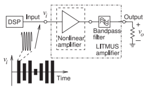
Figure \(\PageIndex{5}\): LITMUS amplifier. Each pulse of the input signal, \(v_{i}\), has many sinusoids. For each pulse the sinusoids have different frequency, amplitude, and relative phase.

combine signals of different frequencies spaced in time. This is a result of the time-frequency behavior of filters, which is discussed in Section 2.18 of [2].

The most common way of reducing distortion of an amplifier is by setting the average output power of a modulated signal at a level that is below the \(1\text{ dB}\) gain compression level by PMEPR. This is called backing off. So while an amplifier, such as a switching amplifier or a Class C amplifier could have close to \(100\%\) efficiency for a signal with a constant envelope, the back-off required for modulated signals with nonconstant envelopes significantly reduces the achievable efficiency.

A digitally modulated signal in a time interval \(\Delta t\) (coinciding with one or a few symbol interval times) can be decomposed into a sum of sinusoids that differ in amplitude, frequency, and relative phase [65]. (Generalizing this, the signal could be represented as a sum of constant envelope signals.) Now each sinusoid can be represented by a CW pulse of duration \(\Delta\tau ≪ \Delta t\) so that each pulse contains \(\Delta\tau /T\) cycles of its sinusoidal constituent, where \(T\) is the period of the sinewave. These pulses can be separated in time, as shown for the input signal, \(v_{i}\), in Figure \(\PageIndex{5}\). This input CW pulse train, generated in the DSP unit, is then applied to the input of the highly efficient nonlinear amplifier, which produces CW pulses at the output of the nonlinear amplifier. The output CW pulses are then combined in the bandpass filter. The bandpass filter spreads the pulses in time and reconstitutes the original, but now amplified, digitally modulated signal. During the time \(\Delta\tau\) of each input pulse, the nonlinear amplifier is amplifying a constant envelope signal so the amplifier can operate in high-efficiency mode and saturation of the nonlinear circuit is not of concern. Also, since the individual frequency components are separated in time in the nonlinear part of the circuit, there can be no intermodulation distortion.

Theoretically a LITMUS amplifier completely suppresses intermodulation distortion, but the suppression achieved is limited by the bandwidth of the pulse train and also limited by reactive and memory effects in the nonlinear amplifier, especially baseband effects (including thermal effects),

The output spectrum following amplification of a signal decomposed into four tones is shown in Figure \(\PageIndex{6}\)(a). Curve (i) is the spectrum of the output of a conventional amplifier and Curve (ii) is the output of a LITMUS amplifier. Both amplifiers produce the same average RF power at the output. The output power of each of the four tones is \(0\text{ dBm}\). In Figure \(\PageIndex{6}\)(a) six intermodulation tones are seen, three below the four fundamental tones and three above. These intermodulation tones are IM3 tones, as their frequencies can be numerically calculated as twice the frequency of one of the fundamental tones minus the frequency of one of the other tones. For

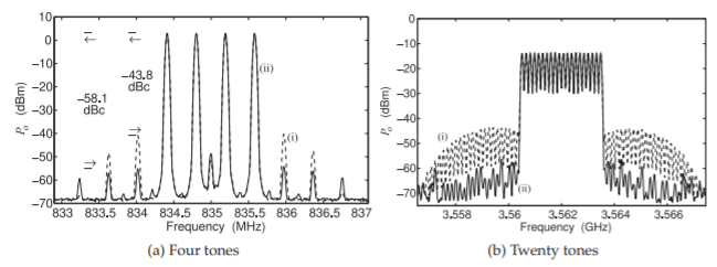
Figure \(\PageIndex{6}\): Measured spectra at the output of the LITMUS amplifier for a different number of input tones. Curve (i) in both figures is the spectrum of the output of a conventional amplifier with a multitone input signal. Curve (ii) is the spectrum of the output of a LITMUS amplifier after the bandpass filter. The spike seen at \(835\text{ MHz}\) is an artifact of the arbitrary waveform generator used to produce the signal. After [64].

the conventional amplifier, the largest intermodulation tone has an output power of \(−43.8\text{ dBm}\). For the LITMUS amplifier the largest intermodulation tone has a power of \(−58.1\text{ dBm}\). The intermodulation distortion is reduced by \(14.3\text{ dB}\).

The amplification of a signal decomposed into \(20\) tones is shown in Figure \(\PageIndex{6}\)(b). Again Curve (i) is the spectrum of the output of a conventional amplifier and Curve (ii) is the output of a LITMUS amplifier for the same output power. Now spectral regrowth is reduced by \(13.9\text{ dB}\).

4.8.5 Summary

There are many variations on the advanced power amplifier architectures discussed in this section. These architectural concepts can be combined with each other and can also be combined with switching amplifier concepts. So the number of different power amplifier conceptual combinations is enormous and many papers have been written about them. Some amplifier topologies require high-performance DSP and high-performance transistors, while others require extensive manual tuning of each amplifier. These affect the cost of each amplifier. Also, the design cost of some amplifiers can be high and require the most experienced designers. These factors are considered in choosing the best amplifier architecture for a particular application.