3.1: OBJECTIVES

Last updated
Save as PDF

Page ID: 58441

James K. Roberge
Massachusetts Institute of Technology via MIT OpenCourseWare

\( \newcommand{\vecs}[1]{\overset { \scriptstyle \rightharpoonup} {\mathbf{#1}} } \) \( \newcommand{\vecd}[1]{\overset{-\!-\!\rightharpoonup}{\vphantom{a}\smash {#1}}} \)\(\newcommand{\id}{\mathrm{id}}\) \( \newcommand{\Span}{\mathrm{span}}\) \( \newcommand{\kernel}{\mathrm{null}\,}\) \( \newcommand{\range}{\mathrm{range}\,}\) \( \newcommand{\RealPart}{\mathrm{Re}}\) \( \newcommand{\ImaginaryPart}{\mathrm{Im}}\) \( \newcommand{\Argument}{\mathrm{Arg}}\) \( \newcommand{\norm}[1]{\| #1 \|}\) \( \newcommand{\inner}[2]{\langle #1, #2 \rangle}\) \( \newcommand{\Span}{\mathrm{span}}\) \(\newcommand{\id}{\mathrm{id}}\) \( \newcommand{\Span}{\mathrm{span}}\) \( \newcommand{\kernel}{\mathrm{null}\,}\) \( \newcommand{\range}{\mathrm{range}\,}\) \( \newcommand{\RealPart}{\mathrm{Re}}\) \( \newcommand{\ImaginaryPart}{\mathrm{Im}}\) \( \newcommand{\Argument}{\mathrm{Arg}}\) \( \newcommand{\norm}[1]{\| #1 \|}\) \( \newcommand{\inner}[2]{\langle #1, #2 \rangle}\) \( \newcommand{\Span}{\mathrm{span}}\)\(\newcommand{\AA}{\unicode[.8,0]{x212B}}\)

The output produced by an operational amplifier (or any other dynamic system) in response to a particular type or class of inputs normally provides the most important characterization of the system. The purpose of this chapter is to develop the analytic tools necessary to determine the response of a system to a specified input.

While it is always possible to determine the response of a linear system to a given input exactly, we shall frequently find that greater insight into the design process results when a system response is approximated by the known response of a simpler configuration. For example, when designing a low-level preamplifier intended for audio signals, we might be interested in keeping the frequency response of the amplifier within \(\pm 5\)% of its mid-band value over a particular bandwidth. If it is possible to approximate the amplifier as a two- or three-pole system, the necessary constraints on pole location are relatively straightforward. Similarly, if an oscilloscope vertical amplifier is to be designed, a required specification might be that the over shoot of the amplifier output in response to a step input be less than 3% of its final value. Again, simple constraints result if the system transfer function can be approximated by three or fewer poles.

The advantages of approximating the transfer functions of linear systems can only be appreciated with the aid of examples. The LM301A integrated-circuit operational amplifier(This amplifier is described in Section 10.4.1.) has 13 transistors included-in its signal-trans mission path. Since each transistor can be modeled as having two capacitors, the transfer function of the amplifier must include 26 poles. Even this estimate is optimistic, since there is distributed capacitance, comparable to transistor capacitances, associated with all of the other components in the signal path.

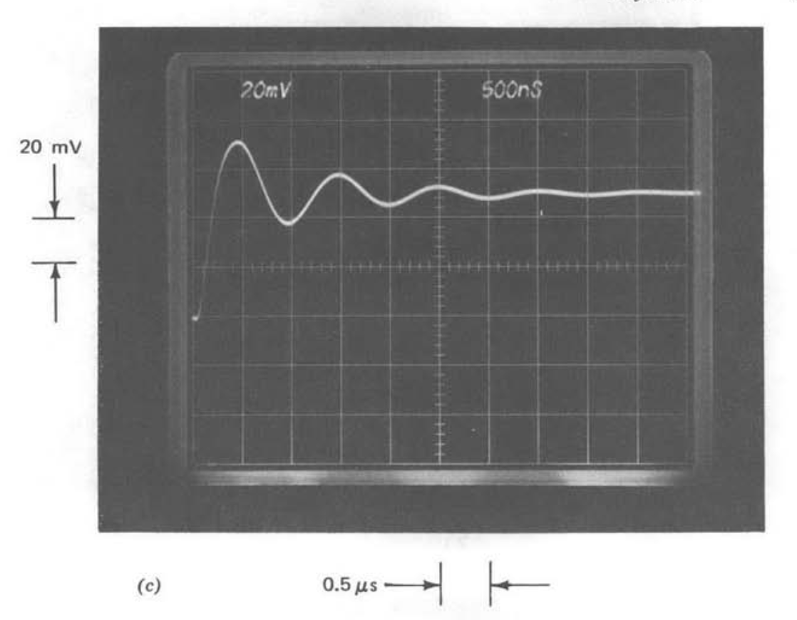
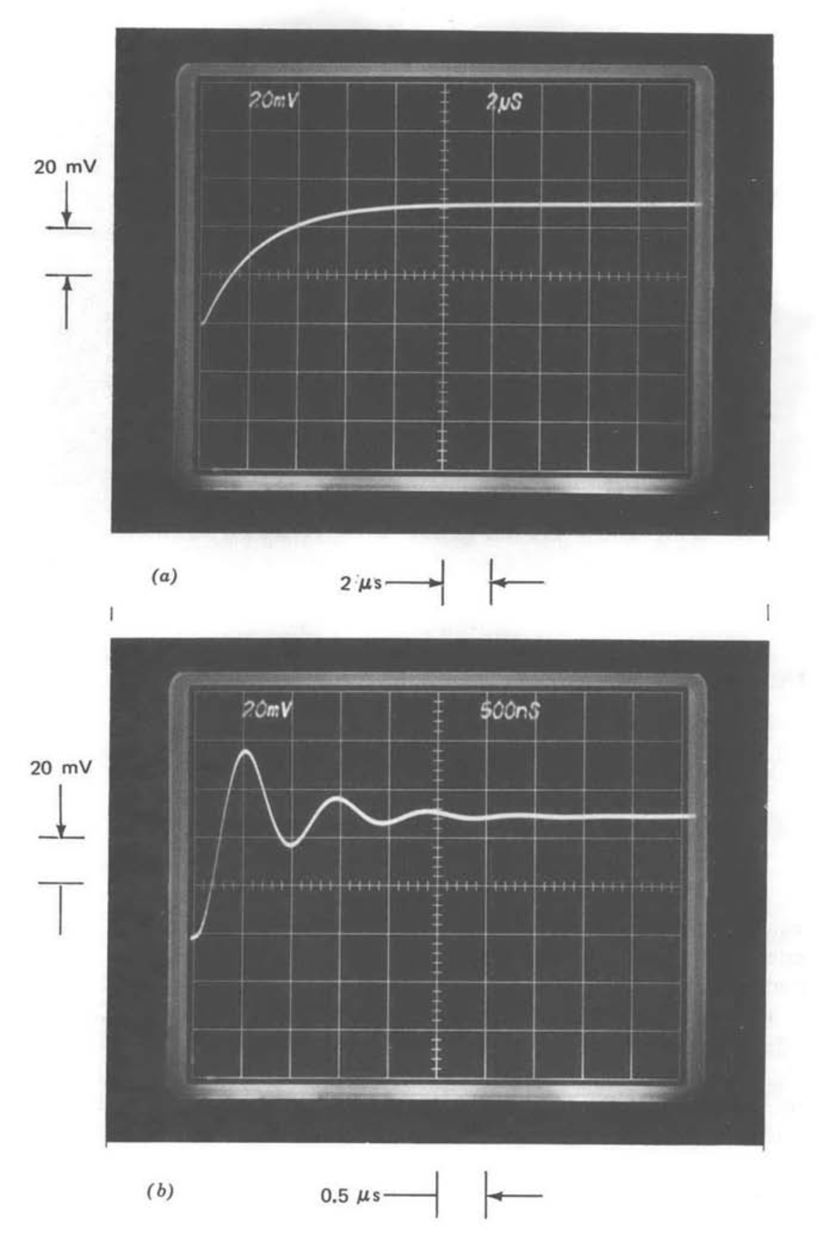
截屏2021-08-05 下午8.38.47.png — Figure 3.1 Step responses of inverting amplifier. (\(a\)) Connection. (\(b\)) Step response with 220-pF compensating capacitor. (\(c\)) Step response with 12-pF compensating 3.1 capacitor.

Fortunately, experimental measurements of performance can save us from the conclusion that this amplifier is analytically intractable. Figure 3.1\(a\) shows the LM301A connected as a unity-gain inverter. Figures 3.1\(b\) and 3.1\(c\) show the output of this amplifier with the input a -50-mV step for two different values of compensating capacitor.(Compensation is a process by which the response of a system can be modified advan tageously, and is described in detail in subsequent sections.) The responses of an \(R-C\) network and an \(R-L-C\) network when excited with +50-mV steps supplied from the same generator used to obtain the previous transients are shown in Figs. 3.2\(a\) and 3.2\(b\), respectively. The network transfer functions are

\[\dfrac{V_o (s)}{V_i (s)} = \dfrac{1}{2.5 \times 10^{-6} s + 1}\label{eq3.1.1} \]

for the response shown in Figure 3.2 \(a\) and

\[\dfrac{V_o (s)}{V_i (s)} = \dfrac{1}{2.5 \times 10^{-14} s^2 + 7 \times 10^{-8} s + 1}\label{eq3.1.2} \]

for that shown in Figure 3.2b. We conclude that there are many applications where the first- and second-order transfer functions of Equations 3.1 and 3.2 adequately model the closed-loop transfer function of the LM301A when connected and compensated as shown in Figure 3.1.

This same type of modeling process can also be used to approximate the open-loop transfer function of the operational amplifier itself. Assume that the input impedance of the LM301A is large compared to 4.7 \(k\Omega\) and that its output impedance is small compared to this value at frequencies of interest. The closed-loop transfer function for the connection shown in Figure 3.1 is then

\[\dfrac{V_o (s)}{V_i (s)} = \dfrac{-a(s)}{2 + a(s)}\label{eq3.1.3} \]

截屏2021-08-05 下午8.44.19.png — Figure 3.2 Step responses for first- and second-order networks. (\(a\)) Step response for \(V_o (s)/V_i (s) = 1/(2.5 \times 10^{-6} s + 1)\). (\(b\)) Step response for \(V_o (s) /V_i (s) = 1/(2.5 \times 10^{-14} s^2 + 7 \times 10^{-8} s + 1)\).

where \(a(s)\) is the unloaded open-loop transfer function of the amplifier. Substituting approximate values for closed-loop gain (the negatives of Equations \(\ref{eq3.1.1}\) and \(\ref{eq3.1.2}\)) into Equation \(\ref{eq3.1.3}\) and solving for \(a(s)\) yields

\[a(s) \simeq \dfrac{8 \times 10^5}{s} \nonumber \]

and

\[a(s) \simeq \dfrac{2.8 \times 10^7}{s(3.5 \times 10^{-7} s + 1)} \nonumber \]

as approximate open-loop gains for the amplifier when compensated with 220-pF and 12-pF capacitors, respectively. We shall see that these approximate values are quite accurate at frequencies where the magnitude of the loop transmission is near unity.