3.3: Transient Response
- Page ID
- 58443

The transient response of an element or system is its output as a function of time following the application of a specified input. The test signal chosen to excite the transient response of the system may be either an input that is anticipated in normal operation, or it may be a mathematical abstraction selected because of the insight it lends to system behavior. Commonly used test signals include the impulse and time integrals of this function.
Selection of Test Inputs
The mathematics of linear systems insures that the same system information is obtainable independent of the test input used, since the transfer function of a system is clearly independent of inputs applied to the system. In practice, however, we frequently find that certain aspects of system performance are most easily evaluated by selecting the test input to accentuate features of interest.
For example, we might attempt to evaluate the d-c gain of an operational amplifier with feedback by exciting it with an impulse and measuring the net area under the impulse response of the amplifier. This approach is mathematically sound, as shown by the following development. Assume that the closed-loop transfer function of the amplifier is \(G(s)\) and that the corresponding impulse response [the inverse transform of \(G(s)\)] is \(g(t)\). The properties of Laplace transforms show that
\[\int_{0}^{t} g(t) dt = \dfrac{1}{s} G(s) \nonumber \]
The final value theorem applied to this function indicates that the net area under impulse response is
\[\lim_{t \to \infty} \int_{0}^{t} g(t) \ dt = \lim_{s \to 0} s \dfrac{1}{s} G(s) = G(0) \nonumber \]
Unfortunately, this technique involves experimental pitfalls. The first of these is the choice of the time function used to approximate an impulse. In order for a finite-duration pulse to approximate an impulse satisfactorily, it is necessary to have(While this statement is true in general, if only the d-c gain of the system is required, any pulse can be used. An extension of the above development shows that the area under the response to any unit-area input is identical to the area under the impulse response.)
\[t_p \ll \dfrac{1}{|s_m|} \nonumber \]
where \(t_p\) is the width of the pulse and \(s_m\) is the frequency of the pole of \(G(s)\) that is located furthest from the origin.
It may be difficult to find a pulse generator that produces pulses narrow enough to test high-frequency amplifiers. Furthermore, the narrow pulse frequently leads to a small-amplitude output with attendant measurement problems. Even if a satisfactory impulse response is obtained, the tedious task of integrating this response (possibly by counting boxes under the output display on an oscilloscope) remains. It should be evident that a far more accurate and direct measurement of d-c gain is possible if a constant input is applied to the amplifier.
Alternatively, high-frequency components of the system response are not excited significantly if slowly time-varying inputs are applied as test inputs. In fact, systems may have high-frequency poles close to the imaginary axis in the \(s\)-plane, and thus border on instability; yet they exhibit well-behaved outputs when tested with slowly-varying inputs.
For systems that have neither a zero-frequency pole nor a zero in their transfer function, the step response often provides the most meaningful evaluation of performance. The d-c gain can be obtained directly by measuring the final value of the response to a unit step, while the initial discontinuity characteristic of a step excites high-frequency poles in the system transfer function. Adequate approximations to an ideal step are provided by rectangular pulses with risetimes
\[t_r \ll \dfrac{1}{|s_m|} \nonumber \]
(\(s_m\) as defined earlier) and widths
\[t_{\omega} \gg \dfrac{1}{|s_n|} \nonumber \]
where \(s_n\) is the frequency of the pole in the transfer function located closest to the origin. Pulse generators with risetimes under 1 ns are available, and these generators can provide useful information about amplifiers with bandwidths on the order of 100 MHz.
Approximating Transient Responses
Examples in Section 3.1 indicated that in some cases it is possible to approximate the transient response of a complex system by using that of a much simpler system. This type of approximation is possible whenever the transfer function of interest is dominated by one or two poles.
Consider an amplifier with a transfer function
\[\dfrac{V_o (s)}{V_i (s)} = \dfrac{a_0 \prod_{i = 1}^{m} (\tau_{zi} s + 1)}{\prod_{j = 1}^{n} (\tau_{pj} s + 1)} \ n > m, \text{ all } \tau > 0 \nonumber \]
The response of this system to a unit-step input is
\[v_o (t) = \mathcal{L}^{-1} \left [\dfrac{1}{s} \dfrac{V_o(s)}{V_i (s)} \right ] = a_o + \sum_{k = 1}^{n} A_k e^{-t/\tau_p k} \nonumber \]
The \(A\)'s obtained from Equation 3.2.6 after slight rearrangement are
\[A_k = -a_0 \dfrac{\prod_{i = 1}^{m} \left (-\dfrac{\tau_{zi}}{\tau_{pk}} + 1 \right )}{\prod_{j = 1,j \ne k}^{n} \left (-\dfrac{\tau_{pj}}{\tau_{pk}} + 1 \right )} \label{eq3.3.8} \]
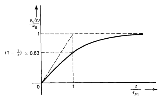
Assume that \(\tau_{p_1} \gg\) all other r's. In this case, which corresponds to one pole in the system transfer function being much closer to the origin than all other singularities, Equation \(\ref{eq3.3.8}\) can be used to show that \(A_1 \simeq a_0\) and all other \(A\)'s \(\simeq 0\) so that
\[v_o (t) \simeq a_0 (1 - e^{-t/\tau_{p_1}}) \nonumber \]
This single-exponential transient response is shown in Figure 3.6. Experience shows that the single-pole response is a good approximation to the actual response if remote singularities are a factor of five further from the origin than the dominant pole.
The approximate result given above holds even if some of the remote singularities occur in complex conjugate pairs, providing that the pairs are located at much greater distances from the origin in the \(s\) plane than the dominant pole. However, if the real part of the complex pair is not more negative than the location of the dominant pole, small-amplitude, high-frequency damped sinusoids may persist after the dominant transient is completed.
Another common singularity pattern includes a complex pair of poles much closer to the origin in the \(s\) plane than all other poles and zeros. An argument similar to that given above shows that the transfer function of an amplifier with this type of singularity pattern can be approximated by the complex pair alone, and can be written in the standard form
\[\dfrac{V_o (s)}{V_i (s)} = \dfrac{a_o}{s^2/\omega_n^2 + 2 \zeta s/\omega_n + 1}\label{eq3.3.10} \]
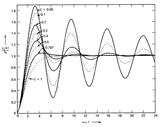
The equation parameters \(\omega_n\) and \(\zeta\) are called the natural frequency (expressed in radians per second) and the damping ratio, respectively. The physical significance of these parameters is indicated in the \(s\)-plane plot shown as Figure 3.7. The relative pole locations shown in this diagram correspond to the underdamped case (\(\zeta < 1\)). Two other possibilities are the critically damped pair (\(\zeta = 1\)) where the two poles coincide on the real axis and the overdamped case (\(\zeta > 1\)) where the two poles are separated on the real axis. The denominator polynomial can be factored into two roots with real coefficients for the later two cases and, as a result, the form shown in Equation \(\ref{eq3.3.10}\) is normally not used. The output provided by the amplifier described by Equation \(\ref{eq3.3.10}\) in response to a unit step is (from Table 3.1).
\[v_o (t) = a_0 \left [1 - \dfrac{1}{\sqrt{1 - \zeta^2}} e^{-\zeta \omega_n t} \sin (\sqrt{1 - \zeta^2} \omega_n t + \Phi) \right ] \nonumber \]
where
\[\Phi = \tan^{-1} \left [\dfrac{\sqrt{1 - \zeta^2}}{\zeta} \right ] \nonumber \]
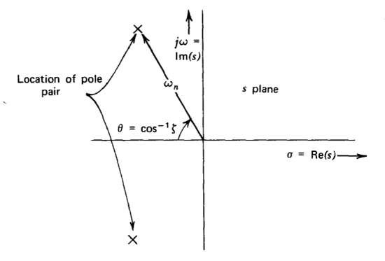
Figure 3.8 is a plot of \(v_o (t)\) as a function of normalized time wat for various values of damping ratio. Smaller damping ratios, corresponding to com plex pole pairs with the poles nearer the imaginary axis, are associated with step responses having a greater degree of overshoot.
The transient responses of third- and higher-order systems are not as easily categorized as those of first- and second-order systems since more parameters are required to differentiate among the various possibilities. The situation is simplified if the relative pole positions fall into certain patterns. One class of transfer functions of interest are the Butterworth filters. These transfer functions are also called maximally flat because of properties of their frequency responses (see Section 3.4). The step responses of Butterworth filters also exhibit fairly low overshoot, and because of these properties feedback amplifiers are at times compensated so that their closed-loop poles form a Butterworth configuration.
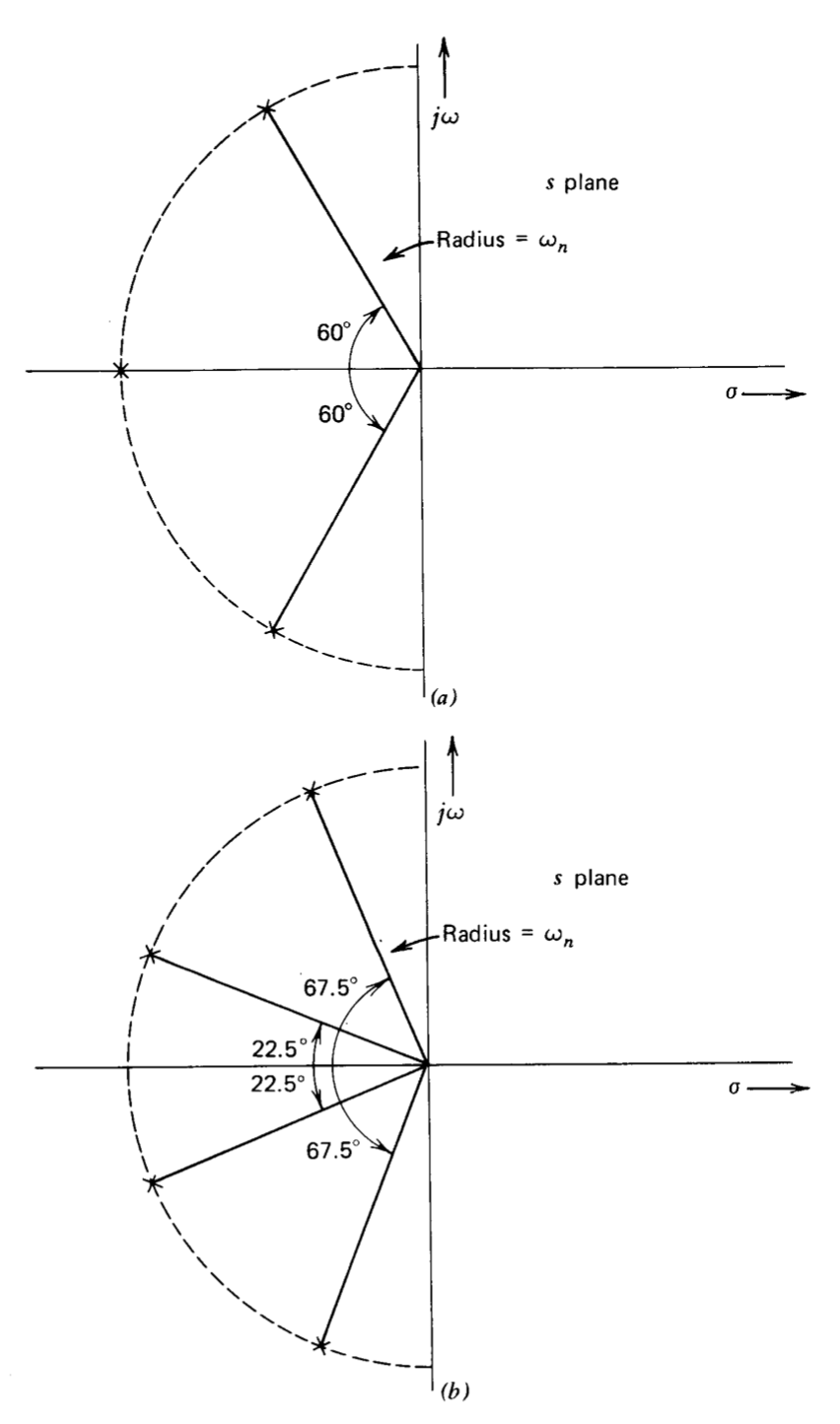
The poles of an nth-order Butterworth filter are located on a circle centered at the origin of the \(s\)-plane. For \(n\) even, the poles make angles \(\pm (2k + 1) 90^{\circ}/n\) with the negative real axis, where k takes all possible integral values from 0 to \((n/2) - 1\). For \(n\) odd, one pole is located on the negative real axis, while others make angles of \(\pm k (180^{\circ}/n)\) with the negative real axis where \(k\) takes integral values from 1 to \((n/2) - (1/2)\). Thus, for example, a first-order Butterworth filter has a single pole located at \(s = - \omega_n\). The second-order Butterworth filter has its poles located \(\pm 45^{\circ}\) from the negative real axis, corresponding to a damping ratio of 0.707.
The transfer functions for third- and fourth-order Butterworth filters are
\[B_3 (s) = \dfrac{1}{s^3/\omega_n^3 + 2s^2/\omega_n^2 + 2s/\omega_n + 1} \nonumber \]
and
\[B_3 (s) = \dfrac{1}{s^4/\omega_n^4 + 2.61 s^3/\omega_n^3 + 3.42 s^2/\omega_n^2 + 2.61 s/\omega_n + 1} \nonumber \]
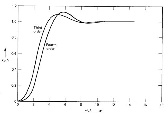
respectively. Plots of the pole locations of these functions are shown in Figure 3.9. The transient outputs of these filters in response to unit steps are shown in Figure 3.10.