1.3: OVERVIEW

The operational amplifier is a powerful, multifaceted analog data-proc­ essing element, and the optimum exploitation of this versatile building block requires a background in several different areas. The primary objec­tive of this book is to help the reader apply operational amplifiers to his own problems. While the use of a "handbook" approach that basically tabulates a number of configurations that others have found useful is attractive because of its simplicity, this approach has definite limitations. Superior results are invariably obtained when the designer tailors the circuit he uses to his own specific, detailed requirements, and to the particular operational amplifier he chooses.

A balanced presentation that combines practical circuit and system design concepts with applicable theory is essential background for the type of creative approach that results in optimum operational-amplifier systems. The following chapters provide the necessary concepts. A second advan­tage of this presentation is that many of the techniques are readily applied to a wide spectrum of circuit and system design problems, and the material is structured to encourage this type of transfer.

Feedback is central to virtually all operational-amplifier applications, and a thorough understanding of this important topic is necessary in any challenging design situation. Chapters 2 through 6 are devoted to feedback concepts, with emphasis placed on examples drawn from operational-amplifier connections. However, the presentation in these chapters is kept general enough to allow its application to a wide variety of feedback sys­tems. Topics covered include modeling, a detailed study of the advantages and limitations of feedback, determination of responses, stability, and com­pensation techniques intended to improve stability. Simple methods for the analysis of certain types of nonlinear systems are also included. This indepth approach is included at least in part because I am convinced that a detailed understanding of feedback is the single most important pre­ requisite to successful electronic circuit and system design.

Several interesting and widely applicable circuit-design techniques are used to realize operational amplifiers. The design of operational-amplifier circuits is complicated by the requirement of obtaining gain at zero fre­quency with low drift and input current. Chapter 7 discusses the design of the necessary d-c amplifiers. The implications of topology on the dynamics of operational-amplifier circuits are discussed in Chapter 8. The design of the high-gain stages used in most modern operational amplifiers and the factors which influence output-stage performance are also included. Chapter 9 illustrates how circuit design techniques and feedback-system concepts are combined in an illustrative operational-amplifier circuit.

The factors influencing the design of the modern integrated-circuit opera­tional amplifiers that have dramatically increased amplifier usage are dis­cussed in Chapter 10. Several examples of representative present-day de­signs are included.

A variety of operational-amplifier applications are sprinkled throughout the first 10 chapters to illustrate important concepts. Chapters 11 and 12 focus on further applications, with major emphasis given to clarifying im­portant techniques and topologies rather than concentrating on minor details that are highly dependent on the specifics of a given application and the amplifier used.

Chapter 13 is devoted to the problem of compensating operational ampli­fiers for optimum dynamic performance in a variety of applications. Dis­cussion of this material is deferred until the final chapter because only then is the feedback, circuit, and application background necessary to fully appreciate the subtleties of compensating modern operational amplifiers available. Compensation is probably the single most important aspect of effectively applying operational amplifiers, and often represents the differ­ence between inadequate and superlative performance. Several examples of the way in which compensation influences the performance of a repre­ sentative integrated-circuit operational amplifier are used to reinforce the theoretical discussion included in this chapter.

PROBLEMS

Exercise \(\PageIndex{1}\)

Design a circuit using a single operational amplifier that provides an ideal input-output relationship

\[V_o = -V_{i1} - 2V_{i2} - 3V_{i3}\nonumber \]

Keep the values of all resistors used between 10 and 100 kU.

Determine the loop transmission (assuming no loading) for your design.

Exercise \(\PageIndex{2}\)

Note that it is possible to provide an ideal input-output relationship

\[V_o = V_{i1} + 2V_{i2} + 3V_{i3}\nonumber \]

by following the design for Problem 1.1 with a unity-gain inverter. Find a more efficient design that produces this relationship using only a single operational amplifier.

Exercise \(\PageIndex{3}\)

An operational amplifier is connected to provide an inverting gain with an ideal value of 10. At low frequencies, the open-loop gain of the ampli­ fier is frequency independent and equal to \(a_0\). Assuming that the only source of error is the finite value of open-loop gain, how large should \(a_0\) be so that the actual closed-loop gain of the amplifier differs from its ideal value by less than 0.1%?

Exercise \(\PageIndex{4}\)

Design a single-amplifier connection that provides the ideal input-output relationship

\[v_o = -100 \int (v_{i1} + v_{i2}) dt \nonumber \]

Figure 1.7 Differential-amplifier connections.

Keep the values of all resistors you use between 10 and 100 \(k\Omega\).

Exercise \(\PageIndex{5}\)

Design a single-amplifier connection that provides the ideal input-output relationship

\[v_o = +100 \int (v_{i1} + v_{i2} ) dt \nonumber \]

using only resistor values between 10 and 100 \(k\Omega\). Determine the loop trans­mission of your configuration, assuming negligible loading.

Exercise \(\PageIndex{6}\)

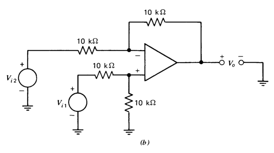
Determine the ideal input-output relationships for the two connections shown in Figure 1.7.

Figure 1.8 Two-pole system.

Exercise \(\PageIndex{7}\)

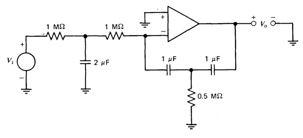
Determine the ideal input-output transfer function for the operational- amplifier connection shown in Figure 1.8. Estimate the value of open-loop gain required such that the actual closed-loop gain of the circuit approaches its ideal value at an input frequency of 0.01 radian per second. You may neglect loading.

Exercise \(\PageIndex{8}\)

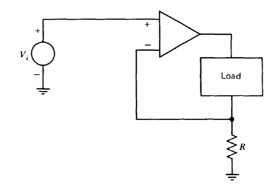
Assume that the operational-amplifier connection shown in Figure 1.9 satisfies the two conditions stated in Section 1.2.2. Use these conditions to determine the output resistance of the connection (i.e., the resistance seen by the load).

Figure 1.9 Circuit with controlled output resistance.

Figure 1.10 Log circuit.

Exercise \(\PageIndex{9}\)

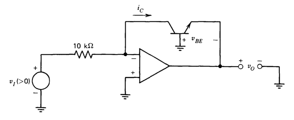
Determine the ideal input-output transfer relationship for the circuit shown in Figure 1.10. Assume that transistor terminal variables are related as

\[i_C = 10^{-13} e^{40v_{BE}}\nonumber \]

where \(i_C\) is expressed in amperes and \(v_{BE}\) is expressed in volts.

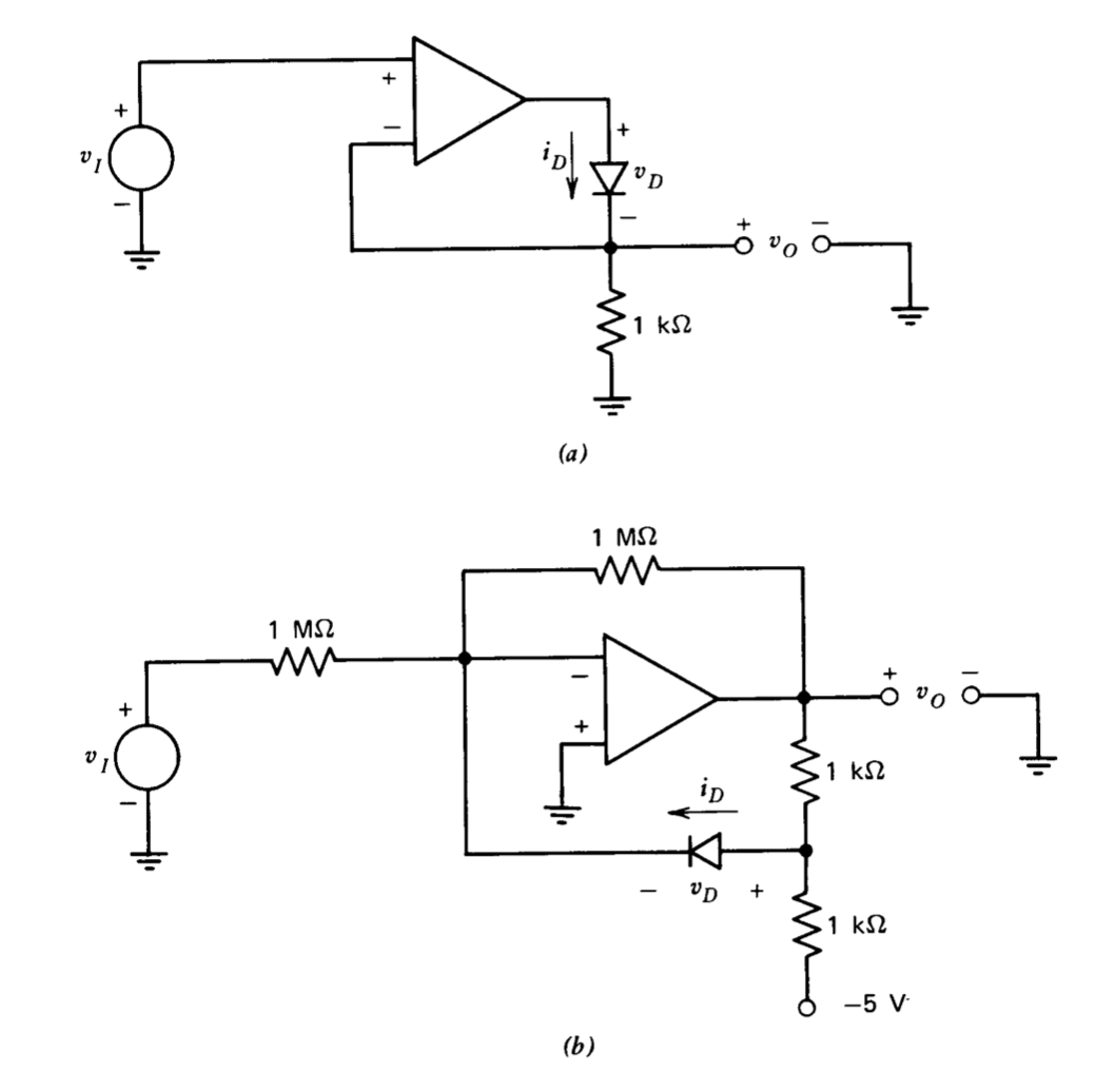
Exercise \(\PageIndex{10}\)

Plot the ideal input-output characteristics for the two circuits shown in Figure 1.11. In part a, assume that the diode variables are related by \(i_D = 10^{-13} e^{40v_D}\), where \(i_D\) is expressed in amperes and \(v_D\) is expressed in volts. In part \(b\), assume that \(i_D = 0\), \(v_D <0\), and \(v_D = 0\), \(i_D > 0\).

Exercise \(\PageIndex{11}\)

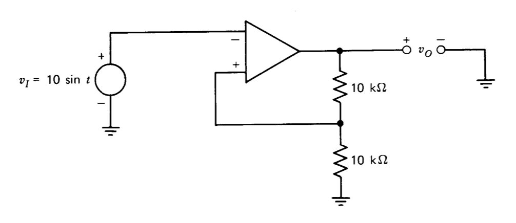
We have concentrated on operational-amplifier connections involving negative feedback. However, several useful connections, such as that shown in Figure 1.12, use positive feedback around an amplifier. Assume that the linear-region open-loop gain of the amplifier is very high, but that its output voltage is limited to \(\pm 10\) volts because of saturation of the ampli­ fier output stage. Approximate and plot the output signal for the circuit shown in Figure 1.12 using these assumptions.

Exercise \(\PageIndex{12}\)

Design an operational-amplifier circuit that provides an ideal input- output relationship of the form

\[v_O = K_1 e^{v_I/K_2}\nonumber \]

where \(K_1\) and \(K_2\) are constants dependent on parameter values used in your design.

Figure 1.11 Nonlinear circuits.

Figure 1.12 Schmitt trigger.