4.3: ROOT-LOCUS TECHNIQUES

A single-loop feedback amplifier is shown in the block diagram of Figure 4.1. The closed-loop transfer function for this amplifier is

\[\dfrac{V_0 (s)}{V_i (s)} = A(s) = \dfrac{a(s)}{1 + a(s) f(s)} \nonumber \]

Root-locus techniques provide a method for finding the poles of the closed- loop transfer function \(A(s)\) [or equivalently the zeros of \(1 + a(s)f(s)\)] given the poles and zeros of \(a(s)f(s)\) and the d-c loop-transmission magnitude \(a_0 f_0\).(If the loop transmission has one or more zeros at the origin so that its d-c magnitude is zero, the closed-loop poles are found from the midband value of \(af\).) Notice that since the quantity \(a_0 f_0\) must appear in one or more terms of the characteristic equation, the locations of the poles of \(A(s)\) must depend on \(a_0f_0\). A root-locus diagram consists of a collection of branches or loci in the s plane that indicate how the locations of the poles of \(A(s)\) change as \(a_0f_0\) varies.

The root-locus diagram provides useful information concerning the performance of a feedback system since the relative stability of any linear system is uniquely determined by its close-loop pole locations. We shall find that approximate root-locus diagrams are easily and rapidly sketched, and that they provide readily interpreted insight into how the closed-loop performance of a system responds to changes in its loop transmission. We shall also see that root-locus techniques can be combined with simple algebraic methods to yield exact answers in certain cases.

Forming the Diagram

A simple example that illustrates several important features of root-locus techniques is provided by the system shown in Figure 4.1 with a feedback transfer function \(f\) of unity and a forward transfer function

\[a(s) = \dfrac{a_0}{(\tau_a s + 1)(\tau_b s + 1)} \nonumber \]

The corresponding closed-loop transfer function is

\[A(s) = \dfrac{a(s)}{1 + a(s) f(s)} = \dfrac{a_0}{\tau_a \tau_b s^2 + (\tau_a + \tau_b) s + (1 + a_0)} \nonumber \]

The closed-loop poles can be determined by factoring the characteristic equation of \(A(s)\), yielding

\[s_1 = \dfrac{-(\tau_a + \tau_b) + \sqrt{(\tau_a + \tau_b)^2 - 4 (1 + a_0) \tau_a \tau_b}}{2 \tau_a \tau_b}\label{eq4.3.4} \]

\[s_2 = \dfrac{-(\tau_a + \tau_b) - \sqrt{(\tau_a + \tau_b)^2 - 4 (1 + a_0) \tau_a \tau_b}}{2 \tau_a \tau_b}\label{eq4.3.5} \]

The root-locus diagram in Figure 4.3 is drawn with the aid of Equation \(\ref{eq4.3.4}\) and \(\ref{eq4.3.5}\). The important features of this diagram include the following.

Figure 4.3 Root-locus diagram for second-order system.

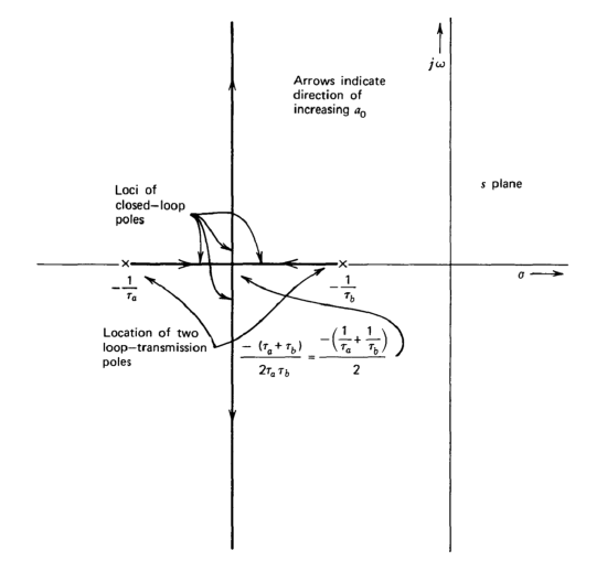
(a) The loop-transmission pole locations are shown. (Loop-transmission zeros are also indicated if they are present.)
(b) The poles of \(A(s)\) coincide with loop-transmission poles for \(a_0 = 0\).
(c) As ao increases, the locations of the poles of \(A(s)\) change along the loci as shown. Arrows indicate the direction of changes that result for increasing \(a_0\).
The two poles coincide at the arithmetic mean of the loop-trans­ mission pole locations for zero radicand in Equation \(\ref{eq4.3.4}\) and \(\ref{eq4.3.5}\), or for
\[a_0 = \dfrac{(\tau_a + \tau_b)^2}{4 \tau_a \tau_b} - 1 \label{eq4.3.6} \]
(e) For increases in ao beyond the value of Equation \(\ref{eq4.3.6}\), the closed-loop pole pair is complex with constant real part and a damping ratio that is a monotonic decreasing function of \(a_0\). Consequently, \(\omega_0\) increases with in­ creasing \(a_0\) in this range.

Certain important features of system behavior are evident from the diagram. For example, the system does not become unstable for any posi­tive value of ao. However, the relative stability decreases as ao increases beyond the value indicated in Equation \(\ref{eq4.3.6}\).

It is always possible to draw a root-locus diagram by directly factoring the characteristic equation of the system under study as in the preceding example. Unfortunately, the effort involved in factoring higher-order poly­nomials makes machine computation mandatory for all but the simplest systems. We shall see that it is possible to approximate the root-locus dia­grams and thus retain the insight often lost with machine computation when absolute accuracy is not required.

The key to developing the rules used to approximate the loci is to realize that closed-loop poles occur only at zeros of the characteristic equation or at frequencies \(s_1\) such that(It is assumed throughout that the system under study is a negative feedback system with the topology shown in Figure 4.1​​​)

\[1 + a(s_1) f(s_1) = 0 \nonumber \]

or

\[a(s_1) f(s_1) = -1 \nonumber \]

Thus, if the point \(s_1\) is a point on a branch of the root-locus diagram, the two conditions

\[|a(s_1) f (s_1)|= -1\label{eq4.3.9} \]

and

\[\measuredangle a(s_1) f(s_1) = (2n + 1) 180^{\circ}\label{eq4.3.10} \]

where \(n\) is any integer, must be satisfied. The angle condition is the more important of these two constraints for purposes of forming a root-locus diagram. The reason is that since we plot the loci as \(a_0f_0\) is varied, it is possible to find a value for a \(a_0f_0\) that satisfies the magnitude condition at any point in the \(s\) plane where the angle condition is satisfied.

By concentrating primarily on the angle condition, we are able to formu­ late a set of rules that greatly simplify root-locus-diagram construction compared with brute-force factoring of the characteristic equation. Here are some of the rules we shall use.

1. The number of branches of the diagram is equal to the number of poles of \(a(s)f(s)\). Each branch starts at a pole of \(a(s)f(s)\) for small values of \(a_0f_0\) and approaches a zero of \(a(s)f(s)\) either in the finite s plane or at infinity for large values of \(a_0f_0\). The starting and ending points are demon­strated by considering

\[a(s) f(s) = a_0 f_0 g(s) \nonumber \]

Figure 4.4 Loci on real axis.

where \(g(s)\) contains the frequency-dependent portion of the loop trans­mission and the value of \(g(0) \triangleq g_0\) is unity. Rearranging Equation \(\ref{eq4.3.9}\),\(\ref{eq4.3.10}\) and using this notation yields

\[|g(s_1)| = \dfrac{1}{a_0 f_0} \nonumber \]

at any point \(s_1\) on a branch of the root-locus diagram. Thus for small values of \(a_0f_0\), \(|g(s_1)|\) must be large, implying that the point si is close to a pole of \(g(s)\). Conversely, a large value of \(a_0f_0\) requires proximity to a zero of \(g(s)\).

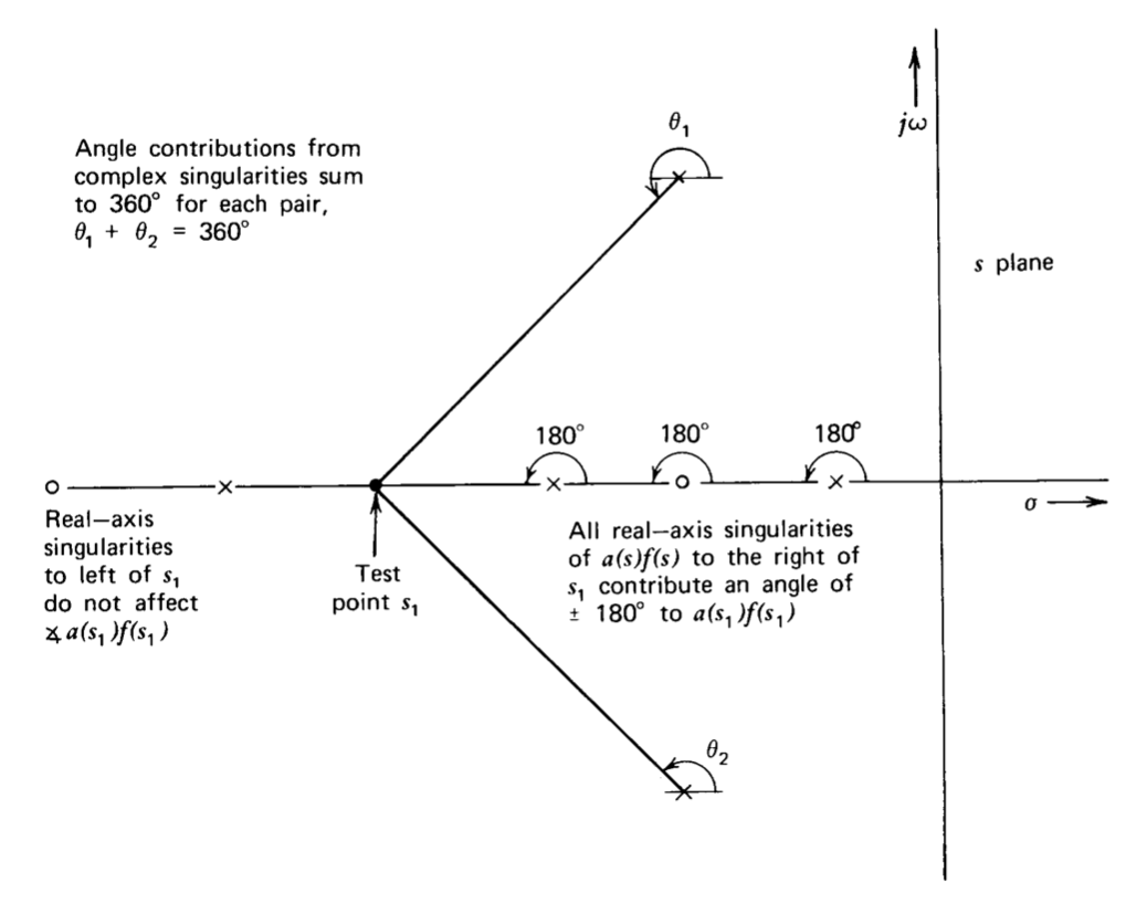
2. Branches of the diagram lie on the real axis to the left of an odd number of real-axis poles and zeros of \(a(s)f(s)\).(Special care is necessary for systems with right-half-plane open-loop singularities. See Section 4.3.3.) This rule follows directly from Equation \(\ref{eq4.3.10}\) as illustrated in Figure 4.4. Each real-axis zero of \(a(s)f(s)\) to the right of \(s_1\) adds \(180^{\circ}\) to the angle of \(a(s_1)f(s_1)\) while each real-axis pole to the right of \(s_1\) subtracts \(180^{\circ}\) from the angle. Real-axis singularities to the left of point \(s_1\) do not influence the angle of \(a(s_1)f(s_1)\). Similarly, since com­plex singularities must always occur in conjugate pairs, the net angle con­tribution from these singularities is zero. This rule is thus sufficient to satisfy Equation \(\ref{eq4.3.10}\). We are further guaranteed that branches must exist on all segments of the real axis to the left of an odd number of singularities of \(a(s)f(s)\), since there is some value of \(a_0f_0\) that will exactly satisfy Equation \(\ref{eq4.3.9}\) at every point on these segments, and the satisfaction of Equations \(\ref{eq4.3.9}\) and \(\ref{eq4.3.10}\) is both necessary and sufficient for the existence of a pole of \(A(s)\).

3. The two separate branches of the diagram that must exist between pairs of poles or pairs of zeros on segments of the real axis that satisfy rule 2 must at some point depart from or enter the real axis at right angles to it. Frequently the precise break-away point is not required in order to sketch the loci to acceptable accuracy. If it is necessary to have an exact location, it can be shown that the break-away points are the solutions of the equation

\[\dfrac{d[g(s)]}{ds} = 0\label{eq4.3.13} \]

for systems without coincident singularities.

4. If the number of poles of \(a(s)f(s)\) exceeds the number of zeros of this function by two or more, the average distance of the poles of \(A(s)\) from the imaginary axis is independent of \(a_0f_0\). This rule evolves from a property of algebraic polynomials. Consider a polynomial

\[\begin{array} {rcl} {P(s)} & = & {(a_1 s + a_1 s_1) (a_2 s + a_2 s_2) (a_3 s + a_3 s_3) \cdots (a_n s + a_n s_n)} \\ {} & = & {(a_1 a_2 \cdots a_n) (s + s_1) (s + s_2) (s + s_3) \cdots (s + s_n)} \\ {} & = & {(a_1 a_2 \cdots a_n) [s^n + (s_1 + s_2 + s_3 + \cdots + s_n) s^{n - 1} + \cdots + s_1 s_2 s_3 \cdots s_n]} \end{array}\label{eq4.3.14} \]

From the final expression of Equation \(\ref{eq4.3.14}\), we see that the ratio of the co­efficients of the \(s^{n-1}\) term and the sn term (denoted as \(-n\bar{s}\)) is

\[-n \bar{n} = s_1 + s_2 + s_3 \cdots + s_n\label{eq4.3.15} \]

Since imaginary components of terms on the right-hand side of Equation \(\ref{eq4.3.15}\) must occur in conjugate pairs and thus cancel, the quantity

\[s = -\dfrac{(s_1 + s_2 + s_3 + \cdots + s_n)}{n}\label{eq4.3.16} \]

is the average distance of the roots of \(P(s)\) from the imaginary axis. In order to apply Equation \(\ref{eq4.3.16}\) to the characteristic equation of a feedback system, assume that

\[a(s) f(s) = a_0 f_0 \dfrac{p(s)}{q(s)} \nonumber \]

Then

\[A(s) = \dfrac{a(s)}{1 + a(s) f(s)} = \dfrac{a(s)}{1 + a_0 f_0 [p(s)/q(s)]} = \dfrac{a(s)q(s)}{q(s) + a_0 f_0 p(s)} \nonumber \]

If the order of \(q(s)\) exceeds that of \(p(s)\) by two or more, the ratio of the co­efficients of the two highest-order terms of the characteristic equation of \(A(s)\) is independent of \(a_0f_0\), and thus the average distance of the poles of \(A(s)\) from the imaginary axis is a constant.

5. For large values of \(a_0f_0\), \(P - Z\) branches approach infinity, where \(P\) and \(Z\) are the number of poles and finite-plane zeros of \(a(s)f(s)\), respec­tively. These branches approach asymptotes that make angles with the real axis given by

\[\theta_n = \dfrac{(2n + 1) 180^{\circ}}{P - Z}\label{eq4.3.19} \]

In Equation \(\ref{eq4.3.19}\), \(n\) assumes all integer values from 0 to \(P - Z - 1\). The asymptotes all intersect the real axis at a point

\[\dfrac{\sum \text{ real parts of poles of } a(s) f(s) - \sum \text{ real parts of zeros of } a(s) f(s)}{P - Z} \nonumber \]

The proof of this rule is left to Problem P4.4.

6. Near a complex pole of \(a(s)f(s)\), the angle of a branch with respect to the pole is

\[\theta_p = 180^{\circ} + \sum \measuredangle z - \sum \measuredangle p \nonumber \]

where \(\sum \measuredangle z\) is the sum of the angles of vectors drawn from all the zeros of \(a(s)f(s)\) to the complex pole in question and \(\sum \measuredangle p\) is the sum of the angles of vectors drawn from all other poles of \(a(s)f(s)\) to the complex pole. Similarly, the angle a branch makes with a loop-transmission zero in the vicinity of the zero is

\[\theta_z = 180^{\circ} - \sum \measuredangle z + \sum \measuredangle p \nonumber \]

These conditions follow directly from Equation \(\ref{eq4.3.10}\).

Figure 4.5 Loci in vicinity of low-frequency singularities.

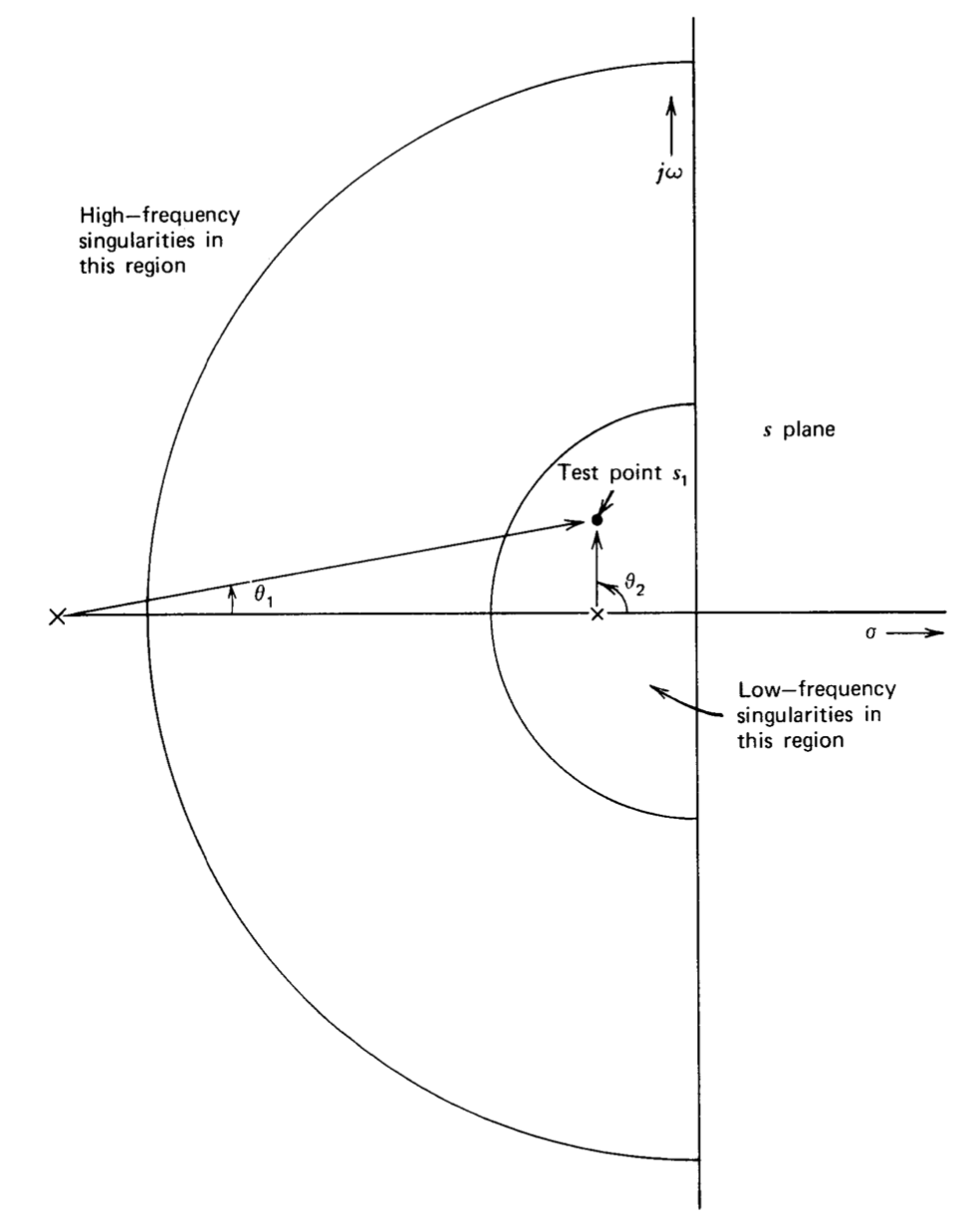
7. If the singularities of \(a(s)f(s)\) include a group much nearer the origin than all other singularities of \(a(s)f(s)\), the higher-frequency singularities can be ignored when determining loci in the vicinity of the origin. Figure 4.5 illustrates this situation. It is assumed that the point si is on a branch if the high-frequency singularities are ignored, and thus the angle of the low-frequency portion of \(a(s)f(s)\) evaluated at \(s = s_1\) must be \((2n + 1)\ 180^{\circ}\). The geometry shows that the angular contribution attributable to remote singularities such as that indicated as \(\theta_1\) is small. (The two angles from a re­mote complex-conjugate pair also sum to a small angle.) Small changes in the location of \(s_1\) that can cause relatively large changes in the angle (e.g., \(\theta_2\)) from low-frequency singularities offset the contribution from remote singularities, implying that ignoring the remote singularities results in in­ significant changes in the root-locus diagram in the vicinity of the low-frequency singularities. Furthermore, all closed-loop pole locations will lie relatively close to their starting points for low and moderate values of \(a_0f_0\). Since the discussion of Section 3.3.2 shows that \(A(s)\) will be dominated by its lowest-frequency poles, the higher-frequency singularities of \(a(s)f(s)\) can be ignored when we are interested in the performance of the system for low and moderate values of \(a_0f_0\).

8. The value of \(a_0f_0\) required to make a closed-loop pole lie at the point \(s_1\) on a branch of the root-locus diagram is

\[a_0 f_0 = \dfrac{1}{|g(s_1)|}\label{eq4.3.22} \]

where \(g(s)\) is defined in rule 1. This rule is required to satisfy Equation \(\ref{eq4.3.9}\).

Examples

The root-locus diagram shown in Figure 4.3 can be developed using the rules given above rather than by factoring the denominator of the closed-loop transfer function. The general behavior of the two branches on the real axis is determined using rules 2 and 3. While the break-away point can be found from Equation \(\ref{eq4.3.13}\), it is easier to use either rule 4 or rule 5 to

establish off-axis behavior. Since the average distance of the closed-loop poles from the imaginary axis must remain constant for this system [the number of poles of \(a(s)f(s)\) is two greater than the number of its zeros], the branches must move parallel to the imaginary axis after they leave the real axis. Furthermore, the average distance must be identical to that for \(a_0f_0 = 0\), and thus the segment parallel to the imaginary axis must be located at \(-\tfrac{1}{2} [(1/\tau_a) + (1/\tau_b)]\). Rule 5 gives the same result, since it shows that the two branches must approach vertical asymptotes that intersect the real axis at \(-\tfrac{1}{2} [(1/\tau_a) + (1/\tau_b)]\).

More interesting root-locus diagrams result for systems with more loop-transmission singularities. For example, the transfer function of an ampli­fier with three common-emitter stages normally has three poles at moderate frequencies and three additional poles at considerably higher frequencies. Rule 7 indicates that the three high-frequency poles can be ignored if this type of amplifier is used in a feedback connection with moderate values of d-c loop transmission. If it is assumed that frequency-independent negative feedback is applied around the three-stage amplifier, a representative af product could be(The corresponding pole locations at - 1, -2, and \(-10\ \text{sec}^{-1}\) are unrealistically low for most amplifiers. These values result, however, if the transfer function for an amplifier with poles at \(- 10^6\), \(- 2 X 10^6\), and \(- 10^7 \text{sec}^{-1}\) is normalized using the microsecond rather than the second as the basic time unit. Such frequency scaling will often be used since it eliminates some of the unwieldy powers of 10 from our calculations.)

\[a(s) f(s) = \dfrac{a_0 f_0}{(s + 1)(0.5s + 1)(0.1s + 1)} \nonumber \]

The root-locus diagram for this system is shown in Figure 4.6. Rule 2 determines the diagram on the real axis, while rule 5 establishes the asymp­totes. Rule 4 can be used to estimate the branches off the real axis, since the branches corresponding to the two lower-frequency poles must move to the right to balance the branch going left from the high-frequency pole. The break-away point can be determined from Equation \(\ref{eq4.3.13}\), with

\[\dfrac{d[g(s)]}{ds} = \dfrac{-[0.15 s^2 + 1.3 s + 1.6]}{[(s + 1) (0.5s + 1) (0.1 s + 1)]^2}\label{eq4.3.24} \]

Zeros of Equation \(\ref{eq4.3.24}\) are at \(- 7.2 \text{sec}^{-1}\) and \(- 1.47 \text{sec}^{-1}\). The higher-frequency location is meaningless for this problem, and in fact corresponds to a break­away point which results if positive feedback is applied around the ampli­fier. Note that the break-away point can be accurately estimated using rule 7. If the relatively higher-frequency pole at \(10 \text{sec}^{-1}\) is ignored, a break-away point at \(- 1.5 \text{sec}^{-1}\) results for the remaining two-pole transfer function.

Algebraic manipulations can be used to obtain more quantitative infor­ mation about the system. Figure 4.6 shows that the system becomes un­ stable as two poles move into the right-half plane for sufficiently large values of \(a_0f_0\). The value of \(a_0f_0\) that moves the pair of closed-loop poles onto the imaginary axis is found by applying Routh's criterion to the characteristic equation of the system, which is (after clearing fractions)

\[\begin{array} {rcl} {P(s)} & = & {(s + 1) (0.5s + 1) (0.1s + 1) + a_0 f_0} \\ {} & = & {0.05s^3 + 0.65 s^2 + 1.6s + 1 + a_0 f_0} \end{array}\label{eq4.3.25} \]

The Routh array is

\[\begin{array} {cc} {0.05} & {1.6} \\ {0.65} & {1 + a_0 f_0} \\ {\dfrac{1}{0.65} (0.99 - 0.05 a_0 f_0)} & {0} \\ {1 + a_0 f_0} & {0} \end{array} \nonumber \]

Two sign reversals indicating instability occur for \(a_0 f_0 > 19.8\). With this value of \(a_0 f_0\), the auxiliary equation is

\[Q(s) = 0.65 s^2 + 20.8 \nonumber \]

The roots of this equation indicate that the poles cross the imaginary axis at \(s = \pm j (5.65)\).

Figure 4.6 Root-locus diagram for third-order system.

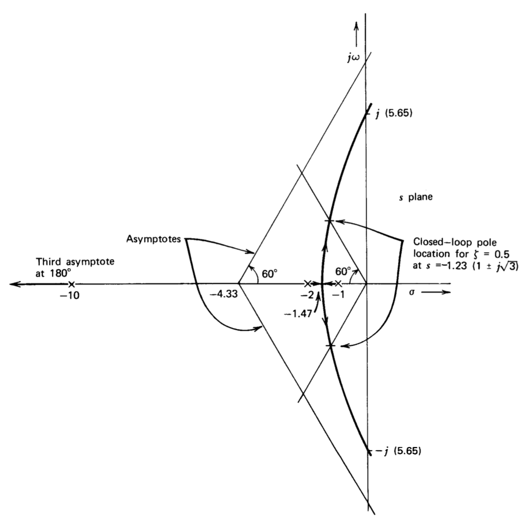
It is also possible to determine values for \(a_0f_0\) that result in specified closed-loop pole configurations. This type of calculation is illustrated by finding the value of \(a_0f_0\) required to provide a damping ratio of 0.5, corre­sponding to complex-pair poles located \(60^{\circ}\) from the real axis. The magni­tude of the ratio of the imaginary part to the real part of the pole location for a pole pair with \(\zeta = 0.5\) is \(\sqrt{3}\). Thus the characteristic equation for this system, when the damping ratio of the complex pole pair is 0.5, is

\[\begin{array} {rcl} {P'(s)} & = & {(s + \gamma )(s + \beta + j \sqrt{3} \beta )(s + \beta - j \sqrt{3} \beta } \\ {} & = & {s^3 + (\gamma + 2\beta )s^2 + 2\beta (\gamma + 2\beta ) s + 4 \gamma \beta^2} \end{array} \nonumber \]

where \(-\gamma\) is the location of the real-axis pole.

The parameters are determined by multiplying Equation \(\ref{eq4.3.25}\) by 20 (to make the coefficient of the \(s^3\) term unity) and equating the new equation to \(P' (s)\).

\[s^3 + 13s^2 + 32 s + 20 (1 + a_0 f_0) = s^3 + (\gamma + 2\beta) s^2 + 2\beta (\gamma + 2\beta )s + 4 \gamma \beta^2\label{eq4.3.29} \]

Equation \(\ref{eq4.3.29}\) is easily solved for \(\gamma , \beta\), and \(a_0f_0\), with the results

Several features of the system are evident from this analysis. Since the complex pair is located at \(s = -1.23 (1 \pm j \sqrt{3})\) when the real-axis pole is located at \(s = - 10.54\), a two-pole approximation based on the pair should accurately model the transient or frequency response of the system. The relatively low desensitivity \(1 + a_0f_0 = 3.2\) results if the damping ratio of the complex pair is made 0.5, and any increase in desensitivity will result in poorer damping. The earlier analysis shows that attempts to increase desensitivity beyond 20.8 result in instability.

Note that since there was only one degree of freedom (the value of \(a_0f_0\)) existed in our calculations, only one feature of the closed-loop pole pattern could be controlled. It is not possible to force arbitrary values for more than one of the three quantities defining the closed-loop pole locations (\(\zeta\) and \(\omega_n\), for the pair and the location of the real pole) unless more degrees of design freedom are allowed.

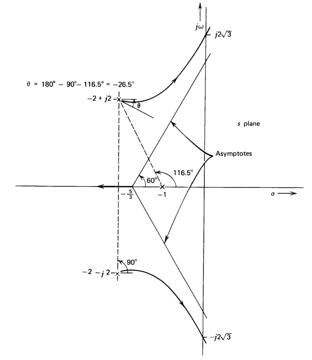
Another example of root-locus diagram construction is shown in Figure 4.7, the diagram for

\[a(s) f(s) = \dfrac{a_0 f_0}{(s + 1)(s^2/8 + s/2 + 1)} \nonumber \]

Rule 5 establishes the asymptotes, while rule 6 is used to determine the loci near the complex poles. The value of \(a_0f_0\) for which the complex pair of poles enters the right-half plane and the frequency at which they cross the imaginary axis are found by Routh's criterion. The reader should verify that these poles cross the imaginary axis at \(s = \pm j 2 \sqrt{3}\) for \(a_0 f_0 = 6.5\).

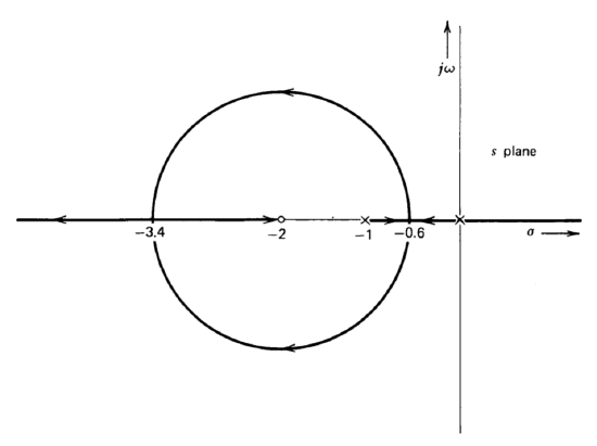
The root-locus diagram for a system with

\[a(s) f(s) = \dfrac{a_0 f_0 (0.5s + 1)}{s (s + 1)} \nonumber \]

Figure 4.7 Root -locus diagram for \(a(s) f(s) = a_0 f_0/[(s + 1) (s^2/8 + s/2 + 1)]\).

is shown in Figure 4.8. Rule 2 indicates that branches are on the real axis between the two loop-transmission poles and to the left of the zero. The points of departure from and reentry to the real axis are obtained by solving

\[\dfrac{d}{ds} \left [ \dfrac{(0.5s + 1)}{(s (s + 1)} \right] = 0 \nonumber \]

yielding \(s = -2 \pm \sqrt{2}\).

Systems With Right-Half-Plane Loop-Transmission Singularities

It is necessary to be particularly careful about the sign of the loop trans­mission when root-locus diagrams are drawn for systems with right-half­-plane loop-transmission singularities. Some systems that are unstable with­ out feedback have one or more loop-transmission poles in the right-half plane. For example, a large rocket does not become aerodynamically stable until it reaches a certain critical speed, and would tip over shortly after lift off if the thrust were not vectored by means of a feedback system. It can be shown that the transfer function of the rocket alone includes a real-axis right-half-plane pole.

Figure 4.8 Root-locus for diagram \(a(s) f(s) = a_0 f_0 (0.5s + 1)/[s(s + 1)]\).

A more familiar example arises from a single-stage common-emitter amplifier. The transfer function of this type of amplifier includes a pole at moderate frequency, a second pole at high frequency, and a high-frequency right-half-plane zero that reflects the signal fed forward from input to output through the collector-to-base capacitance of the transistor. A repre­sentative af product for this type of amplifier with frequency-independent feedback applied around it is

\[a(s) f(s) = \dfrac{a_0 f_0 (-10^{-3} s + 1)}{(10^{-3} s + 1) (s + 1)}\label{eq4.3.34} \]

Figure 4.9 Singularities for common-emitter amplifier.

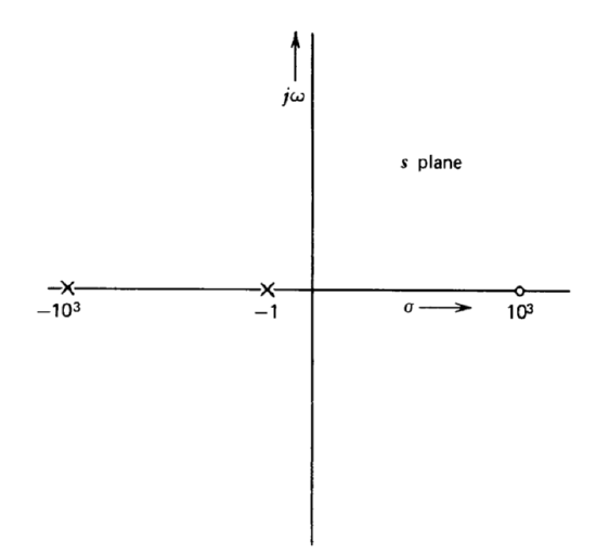
The singularities for this amplifier are shown in Figure 4.9. If the root-locus rules are applied blindly, we conclude that the low-frequency pole moves to the right, and enters the right-half plane for d-c loop-transmission magnitudes in excess of one. Fortunately, experimental evidence refutes this result. The difficulty stems from the sign of the low-frequency gain. It has been assumed throughout this discussion that loop transmission is negative at low frequency so that the system has negative feedback. The rules were developed assuming the topology shown in Figure 4.1 where negative feedback results when \(a_0\) and \(f_0\) have the same sign. If we consider positive feedback systems, Equation \(\ref{eq4.3.10}\) must be changed to

\[\measuredangle a(s_1) f(s_1) = n 360^{\circ} \label{eq4.3.35} \]

where \(n\) is any integer, and rules evolved from the angle condition must be appropriately modified. For example, rule 2 is changed to "branches lie on the real axis to the left of an even number of real-axis singularities for positive feedback systems."

The singularity pattern shown in Figure 4.9 corresponds to a transfer function

\[a'(s) f' (s) = \dfrac{a_0 f_0 (10^{-3}s - 1}{(10^{-3} s + 1)(s + 1)} = \dfrac{-a_0 f_0 (-10^{-3} s + 1)}{(10^{-3} s + 1)(s + 1)} \nonumber \]

because the vector from the zero to \(s = 0\) has an angle of \(180^{\circ}\). The sign reversal associated with the zero when plotted in the \(s\) plane diagram has changed the sign of the d-c loop transmission compared with that of Equation \(\ref{eq4.3.34}\). One way to reverse the effects of this sign change is to substitute Equation \(\ref{eq4.3.35}\) for Equation \(\ref{eq4.3.10}\) and modify all angle-dependent rules accordingly.

A far simpler technique that works equally well for amplifiers with the right-half plane zeros located at high frequencies is to ignore these zeros when forming the root-locus diagram. Since elimination of these zeros eliminates associated sign reversals, no modification of the rules is neces­sary. Rule 7 insures that the diagram is not changed for moderate magni­tudes of loop transmission by ignoring the high-frequency zeros.

Location of Closed-Loop Zeros

A root-locus diagram indicates the location of the closed-loop poles of a feedback system. In addition to the stability information provided by the pole locations, we may need the locations of the closed-loop zeros to determine some aspects of system performance.

The method used to determine the closed-loop zeros is developed with the aid of Figure 4.10. Part \(a\) of this figure shows the block diagram for a single-loop feedback system. The diagram of Figure 4.10\(b\) has the same input-output transfer function as that of Figure 4.10\(a\), but has been modified so that the feedback path inside the loop has unity gain. We first consider the closed-loop transfer function

Figure 4.10. System used to determine closed-loop zeros. (\(a\)) Single-loop feedback system. (\(b\)) Modified block diagram.

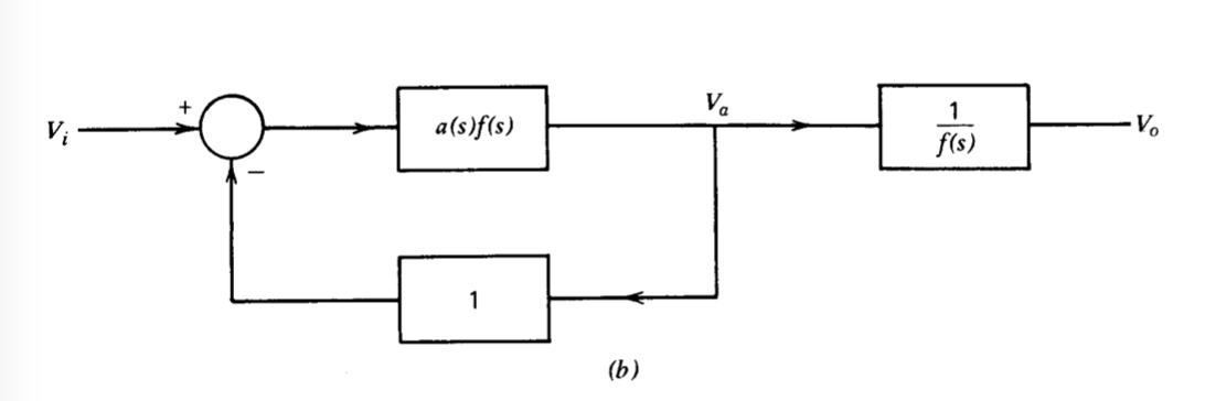
\[\dfrac{V_a (s)}{V_i (s)} = \dfrac{a(s) f(s)}{1 + a(s)f(s)}\label{eq4.3.37} \]

A root-locus diagram gives the pole locations for this closed-loop trans­fer function directly, since the diagram indicates the frequencies at which the denominator of Equation \(\ref{eq4.3.37}\) is zero. The zeros of Equation \(\ref{eq4.3.37}\) coincide with the zeros of the transfer function \(a(s)f(s)\). However, from Figure 4.10\(b\),

\[A(s) = \left [ \dfrac{V_o (s)}{V_i (s)} \right ] = \left [ \dfrac{V_a (s)}{V_i (s)} \right ] \left [ \dfrac{V_o (s)}{V_a (s)} \right ] = \left [ \dfrac{V_a (s)}{V_i (s)} \right ] \left [ \dfrac{1}{f(s)} \right ] \label{eq4.3.38} \]

Thus in addition to the singularities associated with Equation \(\ref{eq4.3.37}\), \(A(s)\) has poles at poles of \(1/f(s)\), or equivalently at zeros of \(f(s)\), and has zeros at poles of \(f(s)\). The additional poles of Equation \(\ref{eq4.3.38}\) cancel the zeros of \(f(s)\) in Equation \(\ref{eq4.3.37}\), with the net result that \(A(s)\) has zeros at zeros of \(a(s)\) and at poles of \(f(s)\). It is important to recognize that the zeros of \(A(s)\) are inde­ pendent of \(a_0f_0\).

An alternative approach is to recognize that zeros of \(A(s)\) occur at zeros of the numerator of this function and at frequencies where the denominator becomes infinite while the numerator remains finite. The later condition is satisfied at poles of \(f(s)\), since this term is included in the denominator of \(A(s)\) but not in its numerator.

Note that the singularities of \(A(s)\) are particularly easy to determine if the feedback path is frequency independent. In this case, (as always) closed-loop poles are obtained directly from the root-locus diagram. The zeros of \(a(s)\), which are the only zeros plotted in the diagram when \(f(s) = f_0\), are also the zeros of \(A(s)\).

These concepts are illustrated by means of two examples of frequency-selective feedback amplifiers. Amplifiers of this type can be constructed by combining twin-\(T\) networks with operational amplifiers. A twin-\(T\) network can have a voltage transfer function that includes complex zeros with posi­tive, negative, or zero real parts. It is assumed that a twin-\(T\) with a voltage-transfer ratio(The transfer function of a twin-T network includes a third real-axis zero, as well as a third pole. Furthermore, none of the poles coincide. The departure from reality repre­sented by Equation \(\ref{eq4.3.39}\) simplifies the following development without significantly changing the conclusions. The reader who is interested in the transfer function of this type of network is referred to J. E. Gibson and F. B. Tuteur, Control System Components, McGraw-Hill, New York, 1958, Section 1.26. )

\[T(s) = \dfrac{s^2 + 1}{s^2 + 2s + 1} \label{eq4.3.39} \]

is available.

Figure 4.11 Rejection amplifier.

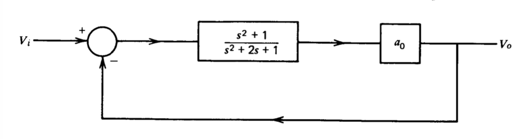
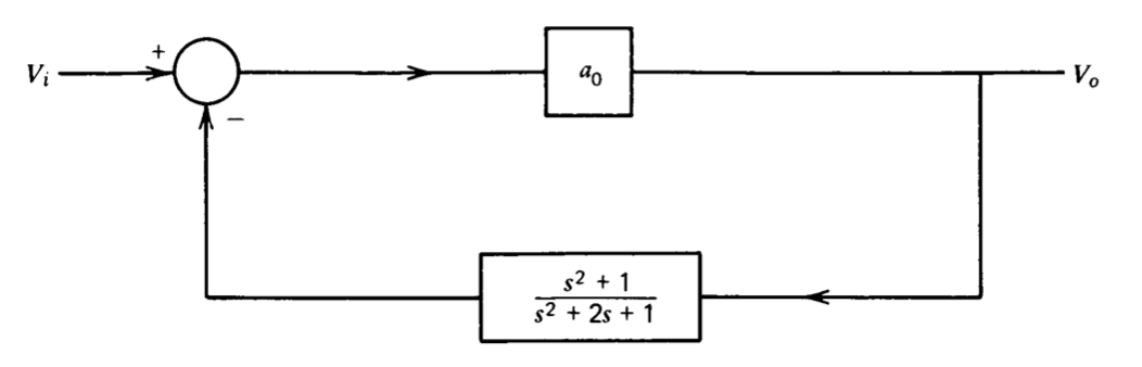
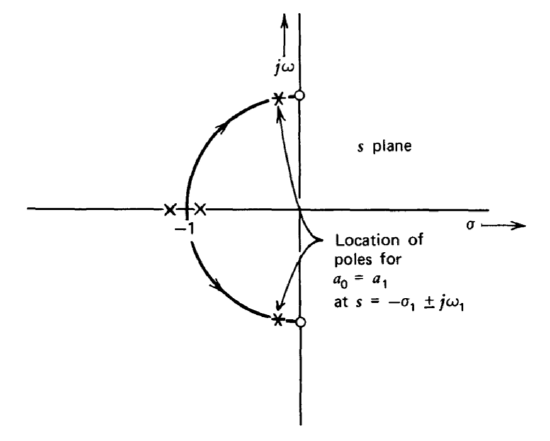
Figures 4.11 and 4.12 show two ways of combining this network with an amplifier that is assumed to have constant gain ao at frequencies of interest. Since both of these systems have the same loop transmission, they have identical root-locus diagrams as shown in Figure 4.13. The closed-loop poles leave the real axis for any finite value of ao and approach the \(j\)-axis zeros along circular arcs. The closed-loop pole location for one particular value of ao is also indicated in this figure.

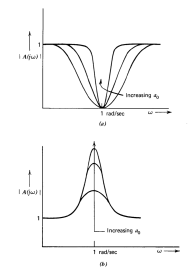
The rejection amplifier (Figure 4.11) is considered first. Since the connection has a frequency-independent feedback path, its closed-loop zeros are the two shown in the root-locus diagram. If the signal Vi is a constant-ampli­tude sinusoid, the effects of the closed-loop poles and zeros very nearly cancel except at frequencies close to one radian per second. The closed-loop frequency response is indicated in Figure 4.14\(a\). As \(a_0\) is increased, the distance between the closed-loop poles and zeros becomes smaller. Thus the band of frequencies over which the poles and zeros do not cancel becomes narrower, implying a sharper notch, as ao is increased.

The bandpass amplifier combines the poles from the root-locus diagram with a second-order closed-loop zero at \(s = - 1\), corresponding to the pole pair of \(f(s)\). The closed-loop transfer function has no other zeros, since \(a(s)\) has no zeros in this connection. The frequency response for this amplifier is shown in Figure 4.14\(b\). In this case the amplifier becomes more selective and provides higher gain at one radian per second as ao increases, since the damping ratio of the complex pole pair decreases.

Figure 4.12 Bandpass amplifier.

Figure 4.13 Root-locus diagram for systems of Figs. 4.11 and 4.12.

Root Contours

The root-locus method allows us to determine how the locations of the closed-loop poles of a feedback system change as the magnitude of the low-frequency loop transmission is varied. There are many systems where relative stability as a function of some parameter other than gain is required. We shall see, for example, that the location of an open-loop singularity in the transfer function of an operational amplifier is frequently varied to compensate the amplifier and thus improve its performance in a given application. Root-locus techniques could be used to plot a family of root- locus diagrams corresponding to various values for a system parameter other than gain. It is also possible to extend root-locus concepts so that the variation in closed-loop pole location as a function of some single param­eter other than gain is determined for a fixed value of \(a_0f_0\). The generalized root-locus diagram that results from this extension is called a root-contour diagram.

In order to see how the root contours are constructed, we recall that the characteristic equation for a negative feedback system can be written in the form

\[P(s) = q(s) = a_0 f_0 p(s) \nonumber \]

where it is assumed that

\[a(s) f(s) = a_0 f_0 \dfrac{p(s)}{q(s)} \nonumber \]

Figure 4.14. Frequency responses for selective amplifiers. (\(a\)) Rejection amplifier. (\(b\)) Bandpass amplifier.

If the \(a_0f_0\) product is constant, but some other system parameter \(\tau\) varies, the characteristic equation can be rewritten

\[P(s) = q'(s) + \tau p'(s) \label{eq4.3.41} \]

All of the terms that multiply \(\tau\) are included in \(p'(s)\) in Equation \(\ref{eq4.3.41}\), so that \(q'(s)\) and \(p'(s)\) are both independent of \(\tau\). The root-contour diagram as a function of \(\tau\) can then be drawn by applying the construction rules to a singularity pattern that has poles at zeros of \(q'(s)\) and zeros at zeros of \(p'(s)\).

An operational amplifier connected as a unity-gain follower is used to illustrate the construction of a root-contour diagram. This connection has unity feedback, and it is assumed that the amplifier open-loop transfer function is

\[a(s) = \dfrac{10^6 (\tau s + 1)}{(s + 1)^2} \nonumber \]

The characteristic equation after clearing fractions is

\[P(s) = s^2 + 2s + (10^6 + 1) + \tau 10^6 s \nonumber \]

Identifying terms in accordance with Equation \(\ref{eq4.3.41}\) results in

\[p' (s) = 10^6 s \nonumber \]

\[q' (s) = s^2 + 2s + 10^6 + 1 \simeq s^2 + 2s + 10^6 \nonumber \]

Figure 4.15 Root-contour diagram for \(p'(s)/q'(s) = 10^6 s/ (s^2 + 2s + 10^6)\).

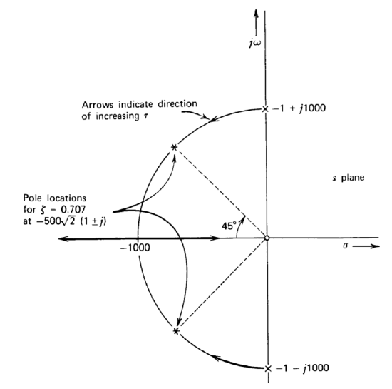
Thus the singularity pattern used to form the root contours has a zero at the origin and complex poles at \(s = - 1 \pm j 10^3\). The root-contour diagram is shown in Figure 4.15. Rule 8 is used to find the value of \(\tau\) necessary to locate the complex pole pair \(45^{\circ}\) from the negative real axis corresponding to a damping ratio of 0.707. From Equation \(\ref{eq4.3.22}\), the required value is

\[\begin{array} {rcl} {\tau} & = & {\left |\dfrac{q'(s)}{p'(s)} \right |_{s = -500 \sqrt{2} (1 + j)}} \\ {} & = & {\left |\dfrac{s^2 + 2s + 10^6}{10^6 s} \right |_{s = -500 \sqrt{2} (1 + j)} = \sqrt{2} \times 10^{-3}} \end{array} \nonumber \]