
5.3: Feedback Compensation
- Page ID
- 58451

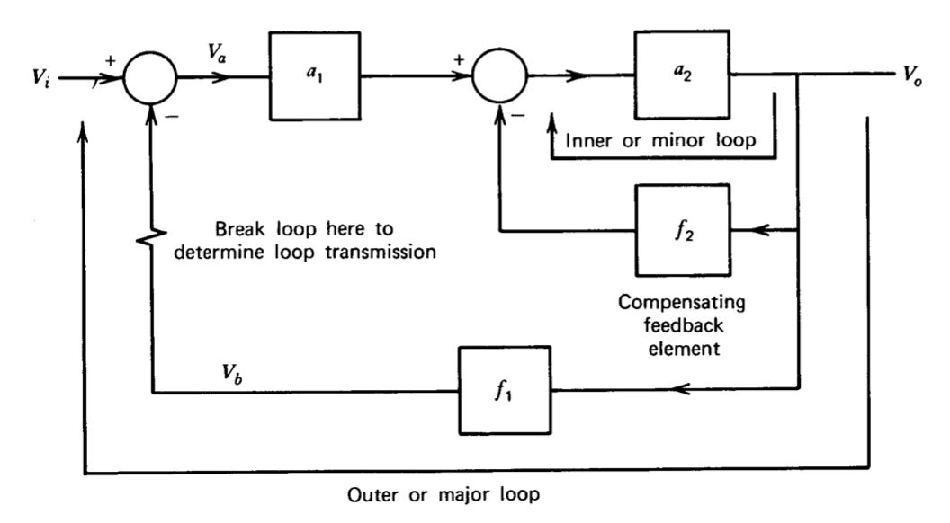
Series compensation is accomplished by adding a cascaded element to a single-loop feedback system. Feedback compensation is implemented by adding a feedback element which creates a two-loop system. One possible topology is illustrated in Figure 5.20. The closed-loop transfer function for this system is
\[\dfrac{V_o}{V_i} = \dfrac{a_1 a_2/(1 + a_2 f_2)}{1 + a_1 a_2f_1/(1 + a_2 f_2)} \nonumber \]
A series-compensated system with a feedback element identical to the major-loop feedback element of Figure 5.20 is shown in Figure 5.21. The two feedback elements are identical since it is assumed that the same ideal closed-loop transfer function is required from the two systems.
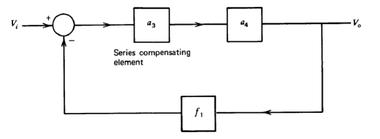
The closed-loop transfer function for the series-compensated system is
\[\dfrac{V_o}{V_i} = \dfrac{a_3 a_4}{1 + a_3 a_4 f_1} \nonumber \]
The closed-loop transfer functions of the feedback- and series-compensated systems will be equal if \(f_2\) is selected so that
\[a_3 = \dfrac{a_1 a_2}{(1 + a_2 f_2) a_4}\label{eq5.3.3} \]
or
\[f_2 = \dfrac{a_1 a_2 - a_3 a_4}{a_2 a_3 a_4}\label{eq5.3.4} \]
The above analysis suggests that one way to select appropriate feedback compensation is first to determine the series compensation that yields acceptable performance and then convert to equivalent feedback compensation. In practice, this approach is normally not used, but rather the series compensation is determined to exploit potential advantages of this method.
We shall see that if an operational amplifier is designed to accept feedback compensation, the use of this technique often results in performance superior to that which can be achieved with series compensation. The frequent advantage of feedback compensation is not a consequence of any error in the mathematics that led to the equivalence of Equation \(\ref{eq5.3.3}\), \(\ref{eq5.3.4}\) but instead is a result of practical factors that do not enter into these calculations. For example, the compensating network required to obtain specified closed-loop performance is often easier to determine and implement and may be less sensitive to variations in other amplifier parameters in the case of a feedback-compensated amplifier. Similarly, problems associated with nonlinearities and noise are often accentuated by series compensation, yet may actually be reduced by feedback compensation.
The approach to finding the type of feedback compensation that should be used in a given application is to consider the negative of the loop trans mission for the system of Figure 5.20. This quantity is
\[\dfrac{V_b}{V_a} = a_1 f_1 \dfrac{a_2}{1 + a_2 f_2} \nonumber \]
If the inner loop is stable (i.e., if \(1 + a_2f_2\) has no zeros in the right half of the \(s\) plane), then
\[\dfrac{V_b (j \omega)}{V_a (j \omega)} \simeq \dfrac{a_1 (j \omega) f_1 (j \omega)}{f_2 (j \omega)} \ \ \ \ |a_2 (j \omega) f_2 (j \omega)| \gg 1\label{eq5.3.6} \]
and
\[\dfrac{V_b (j \omega)}{V_a (j \omega)} \simeq a_1 (j \omega) f_1 (j \omega)a_2 (j \omega) \ \ \ \ |a_2 (j \omega) f_2 (j \omega)| \ll 1\label{eq5.3.7} \]
In practice, system parameters are frequently selected so that the magnitude of the transmission of the minor loop is large at frequencies where the magnitude of the major loop transmission is close to one. The approximation of Equation \(\ref{eq5.3.7}\) can then be used to determine a value for \(f_2\) that insures stability for the system.
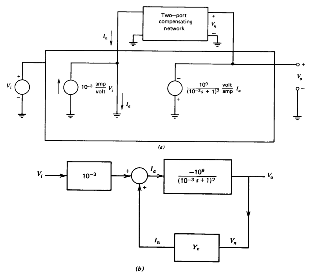
A simple example of feedback compensation is provided by the operational-amplifier model shown in Figure 5.22\(a\). The model is an idealization of a common amplifier topology that will be investigated in detail in subsequent sections. The amplifier modeled includes a first stage with wide bandwidth compared to the rest of the circuit driving into a second stage that has
relatively low input impedance and that dominates the uncompensated dynamics of the amplifier. The compensation is provided by a two-port network that is connected around the second stage and that forms a minor loop. This network is constrained to be passive. A block diagram for the amplifier is shown in Figure 5.22\(b\). The quantity \(Y_c\) is the short-circuit transfer admittance of the compensating network, \(I_n/ V_n\). (The convention used to define \(Y_c\) is at variance with normal two-port notation, which would change the reference direction for \(I_n\). This form is used since it results in fewer minus signs in subsequent equations.)
If no compensation is used, the open-loop transfer function for the amplifier is
\[\dfrac{V_o (s)}{V_i (s)} = -\dfrac{10^6}{(10^{-3} s + 1)^2} \nonumber \]
If a wire is connected from the output of the amplifier back to its input, creating a major loop with \(f = 1\), the phase margin of the resultant system is approximately \(0.12^{\circ}\).
When feedback compensation is included, the block diagram shows that the amplifier transfer function is
\[\dfrac{V_o (s)}{V_i (s)} = \dfrac{-10^6/(10^{-3} s + 1)^2}{1 + 10^9 Y_c/(10^{-3} s + 1)^2}\label{eq5.3.9} \]
One way to improve the phase margin of this amplifier when used in a feedback connection is to make \(V_o (s)/V_i(s)\) dominated by a single pole. Equation \(\ref{eq5.3.9}\) shows that
\[\dfrac{V_o (j\omega)}{V_i (j\omega)} \simeq \dfrac{-10^{-3}}{Y_c (j\omega)} \text{ when } \left | \dfrac{10^9 Y_c (j\omega)}{(10^{-3} j \omega + 1)^2} \right | \gg 1 \nonumber \]
If a single capacitor \(C\) is used for the compensating network, \(Y_c = Cs\) and
\[\dfrac{Y_o (j\omega)}{Y_i (j\omega)} \simeq \dfrac{-10^{-3}}{j \omega C} \nonumber \]
for all frequencies such that
\[\left |\dfrac{10^9 Cj \omega}{(10^{-3} j \omega + 1)^2} \right | \gg 1\nonumber \]
The exact expression for the amplifier open-loop transfer function with this compensation is
\[\dfrac{V_o (s)}{V_i (s)} = \dfrac{-10^6 / (10^{-3} s + 1)^2}{1 + 10^9 Cs/ (10^{-3} s + 1)^2} = \dfrac{-10^6}{10^{-6} s^2 + (2 \times 10^{-3} + 10^9 C)s + 1} \nonumber \]
If an 840-pF capacitor is used for \(C\), the transfer function becomes
\[\dfrac{V_o (s)}{V_i (s)} = \dfrac{-10^6}{(0.84s + 1)(1.19 \times 10^{-6} s + 1)} \nonumber \]
and a phase margin of at least \(45^{\circ}\) is assured for frequency-independent feedback with any magnitude less than one applied around the amplifier. With this value of compensating feedback element,
\[-\dfrac{V_o(j \omega)}{V_i (j \omega)} \simeq \dfrac{1.19 \times 10^6}{j\omega} = \dfrac{10^{-3}}{Cj\omega} = \dfrac{10^{-3}}{Y_c (j\omega)} \nonumber \]
at any frequency between 1.19 radians per second and \(0.84 \times 10^6\) radians per second. The two bounding frequencies are those at which the magnitude of the compensating loop transmission is one. The essential point is that minor-loop feedback controls the transfer function of the amplifier over nearly six decades of frequency. We also note that even though a dominant pole has been created by means of feedback compensation, the unity-gain frequency of the compensated amplifier (approximately \(8 \times 10^5\) radians per second) remains close to the uncompensated value of \(10^6\) radians per second.
Feedback compensation is a powerful and frequently used compensating technique for modern operational amplifiers. Several examples of this type of compensation will be provided after the circuit topologies of representative amplifiers have been described.
PROBLEMS
Exercise \(\PageIndex{1}\)
An operational amplifier has an open-loop transfer function
\[a(s) = \dfrac{2 \times 10^5}{(0.1s + 1)(10^{-5} s + 1)^2}\nonumber \]
Design a connection that uses this amplifier to provide an ideal gain of - 10. Include provision to lower the magnitude of the loop transmission so that the overshoot in response to a unit step is 10%. You may use the curves of Figure 4.26 as an aid to determining the required attenuation.
Exercise \(\PageIndex{2}\)
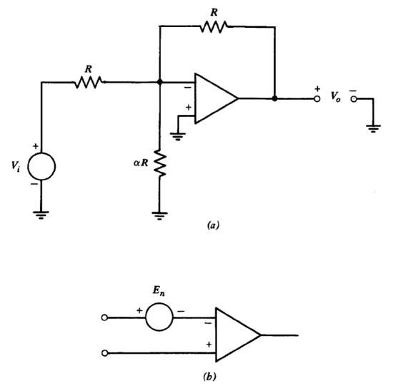
An operational amplifier is connected as shown in Figure 5.23\(a\). The value of \(\alpha\) is adjusted to control the stability of the connection. Assume that noise associated with the amplifier can be modeled as shown in Figure 5.23\(b\). Evaluate the noise at the amplifier output as a function of \(\alpha\), neglecting loading at the input and the output of the amplifier. Note that an increase in the noise at the amplifier output implies a decrease in signal-to-noise ratio, since the gain from input to output is essentially independent of \(\alpha\).
Exercise \(\PageIndex{3}\)
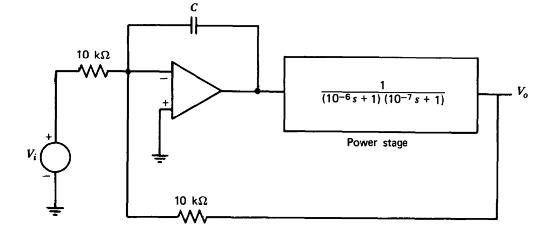
A certain feedback amplifier can be modeled as shown in Figure 5.24. You may assume that the operational amplifier included in this diagram is ideal. Select a value for the capacitor \(C\) that results in a system phase margin of \(45^{\circ}\).
Exercise \(\PageIndex{4}\)
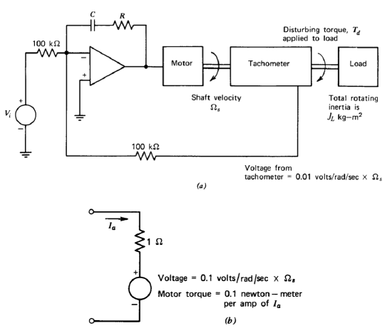
A speed-control system combines a high-power operational amplifier in a loop with a motor and a tachometer as shown in Figure 5.25. The tachometer provides a voltage proportional to output shaft velocity, and this voltage is used as the feedback signal to effect speed control.
- Draw a block diagram for this system that includes the effects of the disturbing torque.
- Determine compensating component values (\(R\) and \(C\)) as a function of \(J_L\) so that the system loop transmission is \(- 100/s\).
- Show that, with this type of loop transmission, the steady-state output velocity is independent of any constant load torque.
- Use an error-coefficient analysis to show that the system is less sensitive to time-varying disturbing torques when larger values of \(J_L\) are used. Assume that \(R\) and \(C\) are changed with \(J_L\) to maintain the loop transmission indicated in part \(b\).
Exercise \(\PageIndex{5}\)
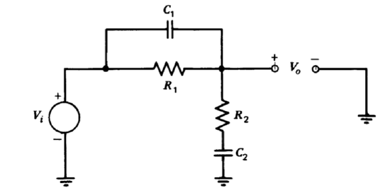
Show that the network illustrated in Figure 5.26 can be used to combine a lag transfer function with a lead transfer function located at a higher frequency. Determine network parameters that will result in the transfer function
\[\dfrac{V_o (s)}{V_i (s)} = \dfrac{(0.1s + 1)(10^{-2} s + 1)}{(s + 1)(10^{-3} s + 1)}\nonumber \]
Exercise \(\PageIndex{6}\)
The loop transmission of a feedback system can be approximated as
\[L(s) = -\dfrac{10^6}{s^2} \nonumber \]
in the vicinity of the unity-gain frequency. Assume that a lead transfer function (Equation 5.2.4) with a value of a = 10 can be added to the loop trans mission. How should the transfer function be located to maximize phase margin? What values of phase margin and crossover frequency result?
Exercise \(\PageIndex{7}\)
Use a block diagram to show that a lag transfer function can be intro duced into the loop transmission of the gain-of-ten amplifier (Figure 5.9) by shunting the \(R\)-valued resistor with an appropriate network.
- Choose network parameters so that the system loop transmission is given by Equation 5.2.17.
- Find the closed-loop transfer function and plot the closed-loop step response for the gain-of-ten amplifier using values found in part \(a\), assuming that the operational-amplifier characteristics are ideal.
- Estimate the closed-loop step response for this connection assuming that the amplifier open-loop transfer function is as given by Equation 5.2.12.
- Compare the performance of the lag-compensated system developed in this problem with that shown in Figure 5.13 considering both the stability and the ideal closed-loop transfer function of the two connections.
Exercise \(\PageIndex{8}\)
It was mentioned in Section 5.2.4 that alternative compensation possibilities for the gain-of-ten amplifier include lowering the magnitude of the loop transmission at all frequencies by a factor of 6.2 and lowering the location of the lowest-frequency pole in the loop transfer function by a factor of 6.2 by selecting appropriate lag-network parameters.
- Determine topologies and component values to implement both of these compensation schemes.
- Draw loop-transmission Bode plots for these two methods of compensation.
- Compare the relative stability produced by these methods with that provided by the lag compensation described in Section 5.2.4.
Exercise \(\PageIndex{9}\)
The negative of the loop transmission for the lead-compensated gain-of ten amplifier described in Section 5.2.4 is
\[a(s)f(s) = \dfrac{5 \times 10^4 (10\tau s + 1)}{(s + 1)(10^{-4} s + 1)(10^{-5} s + 1)(\tau s + 1)}\nonumber \]
where \(\tau\) is determined by the resistor and capacitor values used in the feedback network (see Equation 5.2.15). Use root contours to evaluate the stability of the gain-of-ten amplifier as a function of the parameter \(\tau\). Find the value of \(\tau\) that maximizes the damping ratio of the dominant pole pair. Note. Since it is necessary to factor third- and fourth-order polynomials in order to complete this problem, the use of machine computation is suggested. Numerical calculations are also suggested to evaluate the maximum damping ratio.
Exercise \(\PageIndex{10}\)
The negative of the loop transmission for the lag-compensated amplifier is
\[a(s)f(s) = \dfrac{5 \times 10^4 (\tau s + 1)}{(s + 1)(10^{-4} s + 1)(10^{-5} s + 1)(\alpha \tau s + 1)}\nonumber \]
It was shown in Section 5.2.4 that reasonable stability results for \(\alpha = 6.2\) and a value of \(\tau\) that locates the lag-function zero a factor of 10 below cross over. Use root contours to evaluate stability as a function of the zero location \((1/\tau)\) for \(\alpha = 6.2\). The note concerning the advisability of machine computation mentioned in Problem P5.9 applies to this calculation as well.
Exercise \(\PageIndex{11}\)
Determine the first three error coefficients for the four loop transmissions of the gain-of-ten amplifier described by Equation 5.2.18 through 5.21. Assume that the lead compensation is obtained in the feedback path (see Section 5.2.4) while all other compensations can be considered to be located in the forward path.
Exercise \(\PageIndex{12}\)
A feedback system includes a factor
\[\dfrac{(s^2/12) - (s/2) + 1}{(s^2/12) + (s/2) + 1}\nonumber \]
in its loop transmission.
Assume that you have complete freedom in the choice of d-c loop-transmission magnitude and the selection of additional singularities in the loop transmission. Determine the type of compensation that will maximize the desensitivity of this system.
Exercise \(\PageIndex{13}\)
Calculate the settling time (to 1% of final value for a step input) for the gain-of-ten amplifier with lag compensation (Equation 5.2.17). Contrast this value with that of a first-order system with an identical crossover frequency.
Exercise \(\PageIndex{14}\)
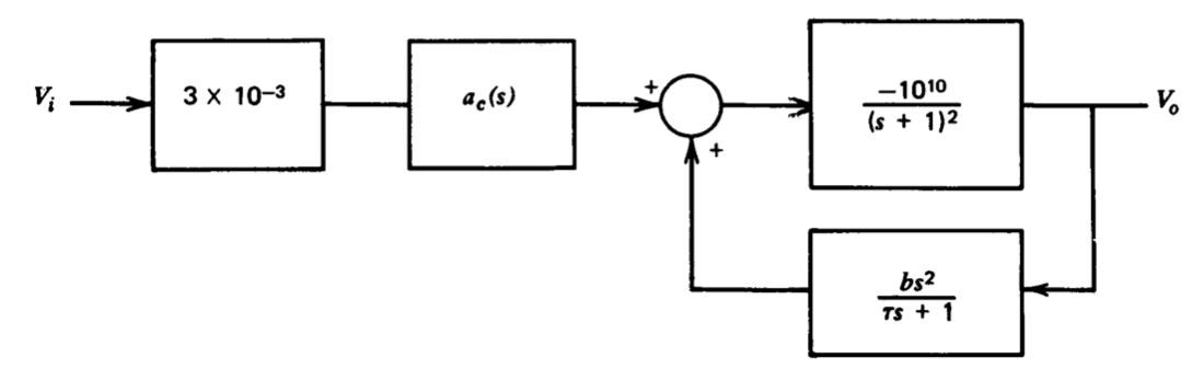
A model for an operational amplifier using minor-loop compensation is shown in block-diagram form in Figure 5.27.
(a) Assume that the series compensating element has a transfer function \(a_c(s) = 1\). Find values for \(b\) and \(\tau\) such that a major loop formed by feeding \(V_o\) directly back to \(V_i\) will have a crossover frequency of \(10^3\) radians per second, approximately \(55^{\circ}\) of phase margin, and maximum desensitivity at frequencies below crossover subject to these constraints. Draw an open-loop Bode plot for the amplifier with these values for \(b\) and \(\tau\).
(b) Now assume that \(b = 0\). Can you find a value for \(a_c(s)\). that results in the same asymptotic open-loop magnitude characteristics as you obtained in part \(a\), subject to the constraint that \(|a_c (j \omega)| \le 1\) for all \(\omega\)?
Exercise \(\PageIndex{15}\)
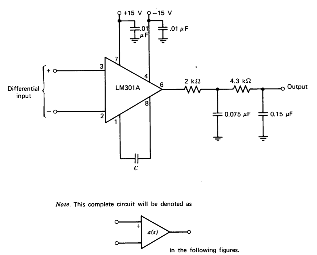
This problem includes a laboratory portion that can be performed with commonly available test equipment and that will give you experience compensating a system with well-defined dynamics. The experimental vehicle is the circuit shown in Figure 5.28, which gives quite repeatable operational-amplifier-like characteristics. The suggested experiments use the configuration at relatively low frequencies, so that the inevitable stray circuit elements have little effect on the measured performance.
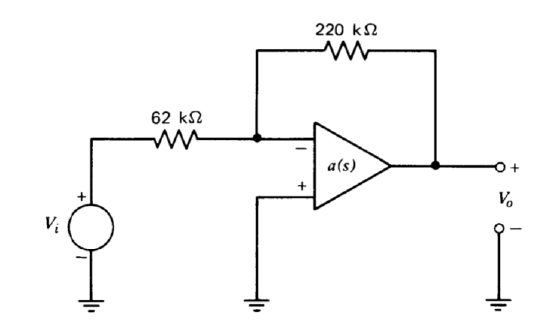
The dynamics of the circuit should first be standardized. Connect it as an inverting amplifier as shown in Figure 5.29.
Select the capacitor \(C\) connected between pins 1 and 8 of the LM301A so that the configuration is just on the verge of instability. An estimated value should be around 5000 pF. Please remember that the amplifier reacts very poorly (usually by dying) if pins 1 or 5 are shorted to almost any potential.
Note. The assumptions required for linear analysis are severely compromised if the peak-to-peak magnitude of the input signal exceeds approximately 50 mV. It is also necessary to have the driving source impedance low in this and other connections. A resistive divider attenuating the signal-generator output and located close to the amplifier is suggested.
After this standardization, it is claimed that if the loads applied to the amplifier are much higher than the output impedance of the network involving the 0.15 \(\mu\)F capacitor, etc., we can approximate \(a(s)\) as
\[a(s) \simeq \dfrac{5 \times 10^4}{(s + 1)(10^{-3}s + 1)(10^{-4} s + 1)} \nonumber \]
for purposes of stability analysis. This transfer function is not unique and, in general, functions of the form
\[a(s) = \dfrac{5 \times 10^4 \tau}{(\tau s + 1)(10^{-3} s + 1)(10^{-4} s + 1)} \nonumber \]
will yield equivalent results in your analysis providing \(\tau \gg 10^{-3}\) seconds. Supply a convincing argument why the above family of transfer functions properly represents the operational amplifier that you have just brought to the verge of oscillation. Note that simply showing the two given expressions are equivalent is not sufficient. You must show why they can be used to analyze the standardized circuit.
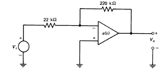
Use a Bode plot to determine the phase margin of the connection shown in Figure 5.30 when the standardized amplifier is used. Predict a value for \(M_p\) based on the phase margin, and compare your prediction with measured results.
You are to compensate the system to improve its phase margin to \(60^{\circ}\) by reducing \(a_0f_0\) and by using lag and lead compensating techniques. You may not change the value of \(C\) or elements in the network connected to the output of the LM301A, nor load the network unreasonably to implement compensation.
Analytically determine the topology and element values you will use for each of the three forms of compensation. It may not be possible to meet the phase-margin objective using lead compensation alone; if you find this to be the case, you may reduce \(a_0f_0\) slightly so that the design goal can be achieved.
Compensate the amplifier in the laboratory and convince yourself that the step responses you measure are reasonable for systems with \(60^{\circ}\) of phase margin. Also correlate the rise times of the responses with your predicted values for crossover frequencies.