
6.2: Linearization
- Page ID
- 58454

One direct and powerful method for the analysis of nonlinear systems involves approximation of the actual system by a linear one. If the approximating system is correctly chosen, it accurately predicts the behavior of the actual system over some restricted range of signal levels. This technique of linearization based on a tangent approximation to a nonlinear relationship is familiar to electrical engineers, since it is used to model many electronic devices. For example, the bipolar transistor is a highly nonlinear element. In order to develop a linear-region model such as the hybrid-pi model to predict the circuit behavior of this device, the relationships between base-to-emitter voltage and collector and base current are linearized. Similarly, if the dynamic performance of the transistor is of interest, linearized capacitances that relate incremental changes in stored charge to incremental changes in terminal voltages are included in the model.
Approximating Function
The tangent approximation is based on the use of a Taylor's series estimation of the function of interest. In general, it is assumed that the output variable of an element is a function of \(N\) input variables
\[v_O = F(v_{I1}, v_{I2}, ..., v_{IN}) \nonumber \]
The output variable is expressed for small variation \(v_{i1}, v_{i2}, ..., v_{iN}\) about input-variable operating points \(V_{I1}, V_{I2}, ..., V_{IN}\) by noting that
\[\begin{array} {rcl} {v_O} & = & {V_O + v_o = F(V_{I1}, V_{I2}, ..., V_{IN})} \\ {} & \ & {+ \sum_{j = 1}^{N} \left.\dfrac{\partial V_O}{\partial V_{Ij}} \right|_{\begin{array} {c} {v_{ij}} \\ {V_{I1}, V_{I2}, ..., V_{IN}} \end{array}}} \\ {} & \ & {+ \dfrac{1}{2!} \sum_{k,l = 1}^{N} \left. \dfrac{\partial^2 V_O}{\partial V_{Ik} \partial V_{Il}} \right |_{\begin{array} {c} {v_{ik}v_{il}} \\ {V_{I1}, V_{I2}, ..., V_{IN}} \end{array}} + \cdots +} \end{array}\label{eq6.2.2} \]
(Recall that the variable and subscript notation used indicates that \(V_o\) is a total variable, \(V_o\) is its operating-point value, and \(v_o\) its incremental component.)
The expansion of Equation \(\ref{eq6.2.2}\) is valid at any operating point where the derivatives exist.
Since the various derivatives are assumed bounded, the function can be adequately approximated by the first-order terms over some restricted range of inputs. Thus
\[V_O + v_o \simeq F(V_{I1}, V_{I2}, ..., V_{IN}) + \sum_{j = 1}^{N} \left. \dfrac{\partial V_O}{\partial V_{Ij}}\right|_{\begin{array} {c} {v_{ij}} \\ {V_{I1}, V_{I2}, ..., V_{IN}} \end{array}}\label{eq6.2.3} \]
The constant terms in Equation \(\ref{eq6.2.3}\) are substracted out, leaving
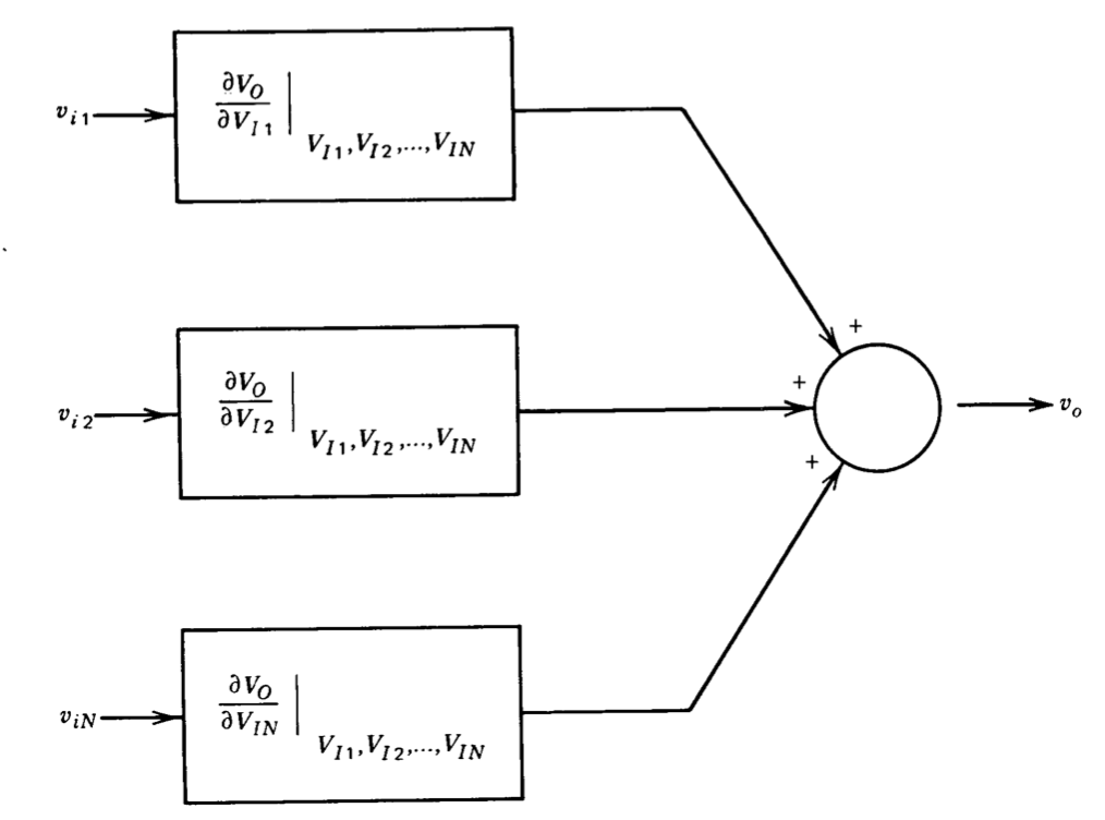
\[v_o \simeq \sum_{j = 1}^{N} \dfrac{\partial V_O}{\partial V_{Ij}}|_{\begin{array} {c} {v_{ij}} \\ {V_{I1}, V_{I2}, ..., V_{IN}} \end{array}}\label{eq6.2.4} \]
Equation \(\ref{eq6.2.4}\) can be used to develop linear-system equations that relate incremental rather than total variables and that approximate the incremental behavior of the actual system over some restricted range of operation. A block diagram of the relationships implied by Equation \(\ref{eq6.2.4}\) is shown in Figure 6.1.
Analysis of an Analog Divider
Certain types of signal-processing operations require that the ratio of two analog variables be determined, and this function can be performed by a divider. Division is frequently accomplished by applying feedback around an analog multiplier, and several commercially available multipliers can be converted to dividers by making appropriate jumpered connections to the output amplifier included in these units. A possible divider connection of this type is shown in Figure 6.2\(a\).
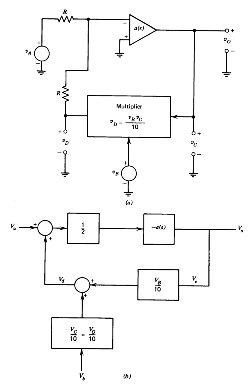
The multiplier scale factor shown in this figure is commonly used since it provides a full-scale output of 10 volts for two 10-volt input signals. It is assumed that the multiplying element itself has no dynamics and thus the speed of response of the system is determined by the operational amplifier.
The ideal relationship between input and output variables can easily be determined using the virtual-ground method. If the current at the inverting input of the amplifier is small and if the magnitude of the loop transmission is high enough so that the voltage at this terminal is negligible, the circuit relationships are
\[v_A + v_D = 0\label{eq6.2.5} \]
and
\[v_D = \dfrac{v_B v_C}{10} = \dfrac{v_Bv_O}{10}\label{eq6.2.6} \]
Solving Equations \(\ref{eq6.2.5}\) and \(\ref{eq6.2.6}\) for \(v_O\) in terms of \(v_A\) and \(v_B\) yields
\[v_O = - \dfrac{10v_A}{v_B} \nonumber \]
System dynamics are determined by linearizing the multiplying-element characteristics. Applying Equation \(\ref{eq6.2.3}\) to the variables of Equation \(\ref{eq6.2.6}\) shows that
\[V_D + v_d \simeq \dfrac{V_B V_C}{10} + \dfrac{V_B v_c}{10} + \dfrac{V_C v_b}{10} \nonumber \]
The incremental portion of this equation is
\[v_d = \dfrac{V_B v_c}{10} + \dfrac{V_c v_b}{10} \nonumber \]
This relationship combined with other circuit constraints (assuming the operational amplifier has infinite input impedance and zero output impedance) is used to develop the incremental block diagram shown in Figure 6.2\(b\).
The incremental dependence of \(V_o\) on \(V_a\), assuming that \(v_B\) is constant, is
\[\dfrac{V_o (s)}{V_a (s)} = \dfrac{-a(s)/2}{1 + V_B a(s)/20}\label{eq6.2.10} \]
If the operational-amplifier transfer function is approximately single pole so that
\[a(s) = \dfrac{a_0}{\tau s + 1} \nonumber \]
and \(a_0\) is very large, Equation \(\ref{eq6.2.10}\) reduces to
\[\dfrac{V_o (s)}{V_a (s)} \simeq \dfrac{-10/V_B}{(20\tau /V_B a_0)s + 1} \nonumber \]
Several features are evident from this transfer function. First, if \(V_B\) is negative, the system is unstable. Second, the incremental step response of the system is first order, with a time constant of \(20\tau / V_Ba_0\) seconds. These features indicate two of the many ways that nonlinearities can affect the performance of a system. The stability of the circuit depends on an input-signal level. Furthermore, if \(V_B\) is positive, the transient response of the circuit becomes faster with increasing \(V_B\), since the loop transmission depends on the value of this input.
Magnetic-Suspension System
An electromechanical system that provides a second example of linearized analysis is illustrated in Figure 6.3. The purpose of the system is to suspend an iron ball in the field of an electromagnet. Only vertical motion of the ball is considered.
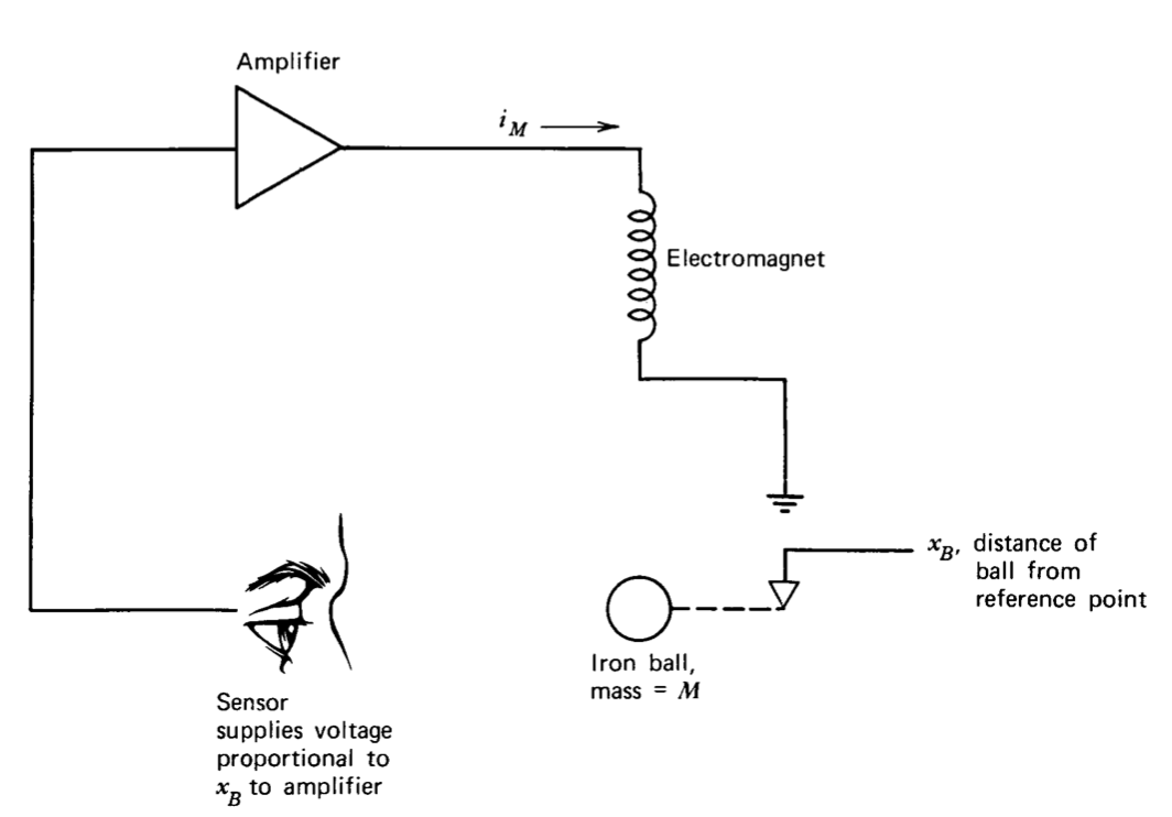
In order to suspend the ball it is necessary to cancel the downward gravitational force on the ball with an upward force produced by the magnet. It is clear that stabilization with constant current is impossible, since while a value of \(x_B\) for which there is no net force on the ball exists, a small deviation from this position changes the magnetic force in such a way as to accelerate the ball further from equilibrium. This effect can be cancelled by appropriately controlling the magnet current as a function of measured ball position.
For certain geometries and with appropriate choice of the reference position for \(x_B\), the magnetic force \(f_M\) exerted on the ball in an upward direction is
\[f_M = \dfrac{Ci_M^2}{x_B^2} \nonumber \]
where \(C\) is a constant.
Assuming incremental changes \(x_b\) and \(i_m\) about operating-point values \(X_B\) and \(I_M\), respectively,
\[f_M = F_M + f_m = \dfrac{CI_M^2}{X_B^2} + \dfrac{2CI_M}{X_B^2} i_m - \dfrac{2CI_M^2}{X_B^3} x_b + \text{ higher-order terms}\label{eq6.2.14} \]
The equation of motion of the ball is
\[\dfrac{Md^2 x_B}{dt^2} = Mg - f_M\label{eq6.2.15} \]
where \(g\) is the acceleration of gravity. Equilibrium or operating-point values are selected so that
\[Mg = \dfrac{CI_M^2}{X_B^2} \nonumber \]
When we combine Equations \(\ref{eq6.2.14}\) and \(\ref{eq6.2.15}\) and assume operation about the equilibrium point, the linearized relationship among incremental variables becomes
\[\dfrac{Md^2 x_b}{dt^2} - \dfrac{2CI_M^2}{X_B^3} x_b = -\dfrac{2CI_M}{X_B^2}i_m\label{eq6.2.17} \]
Equation \(\ref{eq6.2.17}\) is transformed and rearranged as
\[\dfrac{s^2 X_b(s)}{k^2} - X_b (s) = X_b(s) \left (\dfrac{s}{k} + 1 \right ) \left (\dfrac{s}{k} - 1 \right ) = -\dfrac{X_B}{I_M} I_m (s)\label{eq6.2.18} \]
where \(k^2 = 2CI_M^2 / MX_B^3\).
Feedback is applied to the system by making \(i_m\) a linear function of \(x_b\), or
\[I_m (s) = a(s) X_b (s)\label{eq6.2.19} \]
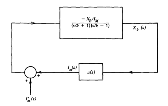
Equations \(\ref{eq6.2.18}\) and \(\ref{eq6.2.19}\) are used to draw the linearized block diagram shown in Figure 6.4. [The input \(I_m'(s)\) is used as a test input later in the analysis.]
The loop transmission for this system
\[L(s) = -\dfrac{a(s) \dfrac{X_B}{I_M}}{\left (\dfrac{s}{k} + 1 \right ) \left (\dfrac{s}{k} - 1 \right )} \nonumber \]
contains a pole in the right-half plane that reflects the fact that the system is unstable in the absence of feedback. A naive attempt at stabilization for this type of system involves cancellation of the right-half-plane pole with a zero of \(a(s)\). While such cancellation works when the singularities in question are in the left-half plane, it is doomed to failure in this case. Although the pole could seemingly be removed from the loop transmission by this method,(Component tolerances preclude exact cancellation in any but a mathematical system.) consider the closed-loop transfer function that relates \(X_b\) to a disturbance \(I_m'\).
If \(a(s)\) is selected as \(a'(s) (s/k - 1)\), this transfer function is
\[\dfrac{X_b (s)}{I_m' (s)} = \dfrac{\dfrac{-X_B/I_M}{(s/k + 1)(s/k - 1)}}{1 + \dfrac{a'(s) X_B/I_M}{s/k + 1}}\label{eq6.2.21} \]
Equation \(\ref{eq6.2.21}\) contains a right-half-plane pole implying exponentially growing responses for Xb even though this growth is not observed as a change in \(i_m\).
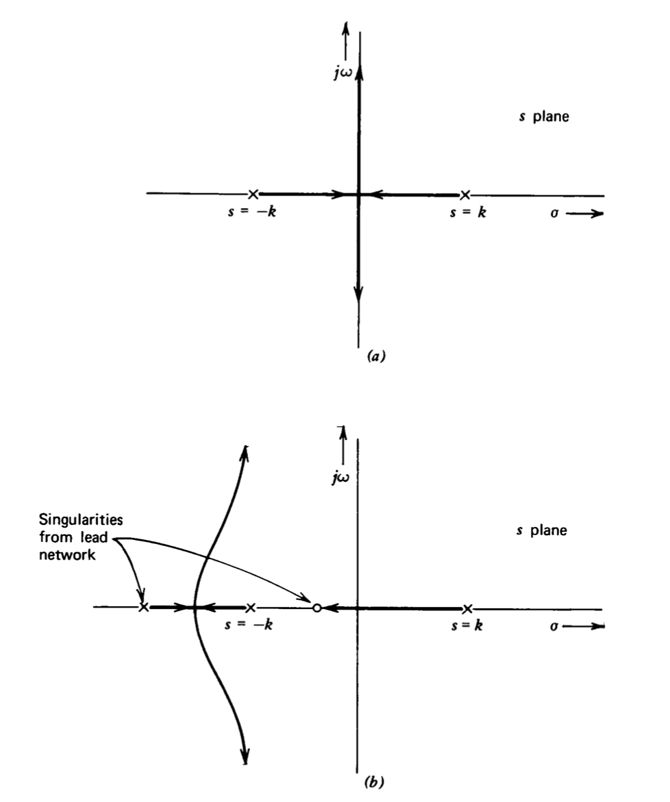
A satisfactory method for compensating the system can be determined by considering the root-locus diagrams shown in Figure 6.5. Figure 6.5\(a\) is the diagram for frequency-independent feedback with \(a(s) = a_0\). As \(a_0\) is increased, the two poles come together and branch out along the imaginary axis. This diagram shows that it is possible to remove the closed-loop pole from the right-half plane if ao is appropriately chosen. However, the poles cannot be moved into the left-half plane, and thus the system exhibits undampened oscillatory responses. The system can be stabilized by including a lead transfer function in \(a(s)\). It is possible to move all closed-loop poles to the left-half plane for any lead-network parameters coupled with a sufficiently high value of \(a_0\). Figure 6.5\(b\) illustrates the root trajectories for one possible choice of lead-network singularities.