3.7: Problems
- Page ID
- 28552
\( \newcommand{\vecs}[1]{\overset { \scriptstyle \rightharpoonup} {\mathbf{#1}} } \)
\( \newcommand{\vecd}[1]{\overset{-\!-\!\rightharpoonup}{\vphantom{a}\smash {#1}}} \)
\( \newcommand{\id}{\mathrm{id}}\) \( \newcommand{\Span}{\mathrm{span}}\)
( \newcommand{\kernel}{\mathrm{null}\,}\) \( \newcommand{\range}{\mathrm{range}\,}\)
\( \newcommand{\RealPart}{\mathrm{Re}}\) \( \newcommand{\ImaginaryPart}{\mathrm{Im}}\)
\( \newcommand{\Argument}{\mathrm{Arg}}\) \( \newcommand{\norm}[1]{\| #1 \|}\)
\( \newcommand{\inner}[2]{\langle #1, #2 \rangle}\)
\( \newcommand{\Span}{\mathrm{span}}\)
\( \newcommand{\id}{\mathrm{id}}\)
\( \newcommand{\Span}{\mathrm{span}}\)
\( \newcommand{\kernel}{\mathrm{null}\,}\)
\( \newcommand{\range}{\mathrm{range}\,}\)
\( \newcommand{\RealPart}{\mathrm{Re}}\)
\( \newcommand{\ImaginaryPart}{\mathrm{Im}}\)
\( \newcommand{\Argument}{\mathrm{Arg}}\)
\( \newcommand{\norm}[1]{\| #1 \|}\)
\( \newcommand{\inner}[2]{\langle #1, #2 \rangle}\)
\( \newcommand{\Span}{\mathrm{span}}\) \( \newcommand{\AA}{\unicode[.8,0]{x212B}}\)
\( \newcommand{\vectorA}[1]{\vec{#1}} % arrow\)
\( \newcommand{\vectorAt}[1]{\vec{\text{#1}}} % arrow\)
\( \newcommand{\vectorB}[1]{\overset { \scriptstyle \rightharpoonup} {\mathbf{#1}} } \)
\( \newcommand{\vectorC}[1]{\textbf{#1}} \)
\( \newcommand{\vectorD}[1]{\overrightarrow{#1}} \)
\( \newcommand{\vectorDt}[1]{\overrightarrow{\text{#1}}} \)
\( \newcommand{\vectE}[1]{\overset{-\!-\!\rightharpoonup}{\vphantom{a}\smash{\mathbf {#1}}}} \)
\( \newcommand{\vecs}[1]{\overset { \scriptstyle \rightharpoonup} {\mathbf{#1}} } \)
\( \newcommand{\vecd}[1]{\overset{-\!-\!\rightharpoonup}{\vphantom{a}\smash {#1}}} \)
\(\newcommand{\avec}{\mathbf a}\) \(\newcommand{\bvec}{\mathbf b}\) \(\newcommand{\cvec}{\mathbf c}\) \(\newcommand{\dvec}{\mathbf d}\) \(\newcommand{\dtil}{\widetilde{\mathbf d}}\) \(\newcommand{\evec}{\mathbf e}\) \(\newcommand{\fvec}{\mathbf f}\) \(\newcommand{\nvec}{\mathbf n}\) \(\newcommand{\pvec}{\mathbf p}\) \(\newcommand{\qvec}{\mathbf q}\) \(\newcommand{\svec}{\mathbf s}\) \(\newcommand{\tvec}{\mathbf t}\) \(\newcommand{\uvec}{\mathbf u}\) \(\newcommand{\vvec}{\mathbf v}\) \(\newcommand{\wvec}{\mathbf w}\) \(\newcommand{\xvec}{\mathbf x}\) \(\newcommand{\yvec}{\mathbf y}\) \(\newcommand{\zvec}{\mathbf z}\) \(\newcommand{\rvec}{\mathbf r}\) \(\newcommand{\mvec}{\mathbf m}\) \(\newcommand{\zerovec}{\mathbf 0}\) \(\newcommand{\onevec}{\mathbf 1}\) \(\newcommand{\real}{\mathbb R}\) \(\newcommand{\twovec}[2]{\left[\begin{array}{r}#1 \\ #2 \end{array}\right]}\) \(\newcommand{\ctwovec}[2]{\left[\begin{array}{c}#1 \\ #2 \end{array}\right]}\) \(\newcommand{\threevec}[3]{\left[\begin{array}{r}#1 \\ #2 \\ #3 \end{array}\right]}\) \(\newcommand{\cthreevec}[3]{\left[\begin{array}{c}#1 \\ #2 \\ #3 \end{array}\right]}\) \(\newcommand{\fourvec}[4]{\left[\begin{array}{r}#1 \\ #2 \\ #3 \\ #4 \end{array}\right]}\) \(\newcommand{\cfourvec}[4]{\left[\begin{array}{c}#1 \\ #2 \\ #3 \\ #4 \end{array}\right]}\) \(\newcommand{\fivevec}[5]{\left[\begin{array}{r}#1 \\ #2 \\ #3 \\ #4 \\ #5 \\ \end{array}\right]}\) \(\newcommand{\cfivevec}[5]{\left[\begin{array}{c}#1 \\ #2 \\ #3 \\ #4 \\ #5 \\ \end{array}\right]}\) \(\newcommand{\mattwo}[4]{\left[\begin{array}{rr}#1 \amp #2 \\ #3 \amp #4 \\ \end{array}\right]}\) \(\newcommand{\laspan}[1]{\text{Span}\{#1\}}\) \(\newcommand{\bcal}{\cal B}\) \(\newcommand{\ccal}{\cal C}\) \(\newcommand{\scal}{\cal S}\) \(\newcommand{\wcal}{\cal W}\) \(\newcommand{\ecal}{\cal E}\) \(\newcommand{\coords}[2]{\left\{#1\right\}_{#2}}\) \(\newcommand{\gray}[1]{\color{gray}{#1}}\) \(\newcommand{\lgray}[1]{\color{lightgray}{#1}}\) \(\newcommand{\rank}{\operatorname{rank}}\) \(\newcommand{\row}{\text{Row}}\) \(\newcommand{\col}{\text{Col}}\) \(\renewcommand{\row}{\text{Row}}\) \(\newcommand{\nul}{\text{Nul}}\) \(\newcommand{\var}{\text{Var}}\) \(\newcommand{\corr}{\text{corr}}\) \(\newcommand{\len}[1]{\left|#1\right|}\) \(\newcommand{\bbar}{\overline{\bvec}}\) \(\newcommand{\bhat}{\widehat{\bvec}}\) \(\newcommand{\bperp}{\bvec^\perp}\) \(\newcommand{\xhat}{\widehat{\xvec}}\) \(\newcommand{\vhat}{\widehat{\vvec}}\) \(\newcommand{\uhat}{\widehat{\uvec}}\) \(\newcommand{\what}{\widehat{\wvec}}\) \(\newcommand{\Sighat}{\widehat{\Sigma}}\) \(\newcommand{\lt}{<}\) \(\newcommand{\gt}{>}\) \(\newcommand{\amp}{&}\) \(\definecolor{fillinmathshade}{gray}{0.9}\)3.7.1: Review Questions
1. Give two examples of how negative feedback is used in everyday life.
2. What circuit parameters will negative feedback alter, and to what extent?
3. What is meant by the term “Sacrifice Factor”?
4. What is the usage of Gain and Phase Margin?
5. Name the different negative feedback connections (i.e., variants or forms).
6. How might negative feedback accidentally turn into positive feedback?
7. What circuit parameters won't negative feedback effect?
8. In practical amplifiers, when does negative feedback “stop working”, and why?
3.7.2: Problems
Analysis Problems
1. An amplifier's open-loop gain plot is given in Figure \(\PageIndex{1}\). If the amplifier is set up for a closed-loop gain of 100, what is the sacrifice factor (\(S\)) at low frequencies? What is \(S\) at 1 kHz?
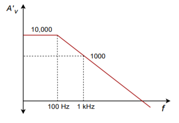
Figure \(\PageIndex{1}\)
2. If the amplifier in Problem 1 has an open-loop THD of 5%, what is the closed-loop THD at low frequencies? Assuming that the open-loop THD doesn't change with frequency, what is the closed-loop THD at 1 kHz?
3. If an amplifier has an open-loop response as given in Figure \(\PageIndex{1}\), and a feedback factor (\(\beta\)) of 0.05 is used, what is the exact low frequency closed loop gain? What is the approximate low frequency gain? What is the approximate gain at 1 kHz?
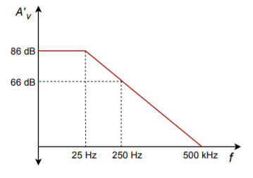
Figure \(\PageIndex{2}\)
4. Using the open loop response curve in Figure \(\PageIndex{2}\), determine exact and approximate values of \(\beta\) for a closed-loop gain of 26 dB.
5. Determine the closed-loop \(f_2\) for the circuit of Problem 4.
6. What is the maximum allowable phase shift at 500 kHz for stable usage of negative feedback in Figure \(\PageIndex{2}\)?
7. Determine the gain and phase margins for the amplifier response given in Figure \(\PageIndex{3}\). Is this amplifier a good candidate for negative feedback?
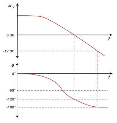
Figure \(\PageIndex{3}\)
8. Determine the closed-loop (mid-band) gain in Figure \(\PageIndex{4}\).
9. What is the closed-loop \(Z_{in}\) in Figure \(\PageIndex{4}\)? What is \(Z_{out}\)?
10. What is the low-frequency sacrifice factor in Figure \(\PageIndex{4}\)?
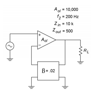
Figure \(\PageIndex{4}\)
11. How much distortion reduction can we hope for in Figure \(\PageIndex{4}\)?
12. How much of a signal/noise improvement can we expect in Figure \(\PageIndex{4}\)?
13. Assuming \(V_{in}(t) = 0.1 \sin 2 \pi 500t\), in Figure \(\PageIndex{4}\), what is \(V_{out}(t)\)?
14. If the circuit in Figure \(\PageIndex{4}\) had an open-loop \(f_1\) of 10 Hz, what would the closed-loop \(f_1\) be?
15. Determine an appropriate pair of resistors to set \(\beta\) to 0.1 in Figure \(\PageIndex{4}\).
Challenge Problems
16. If the feedback network of Figure \(\PageIndex{4}\) produces a phase shift of -200\(^{\circ}\) at 4 kHz, what effect will this have on circuit operation in Problem 10?
17. Consider the circuit of Figure 3.4.4. In general, what effect will the following alterations to the feedback network have on the closed loop system response? A) Placing a capacitor across \(R_f\) B) Placing a capacitor across \(R_i\) C) Placing a rectifying diode across \(R_f\) (both polarities).
Computer Simulation Problems
18. Rerun the simulation of Figure 3.4.5 using the following open loop gains: 1 k, 10 k, and 100 k. What can you conclude from the results?
19. Verify the results of Problem 13 using a circuit simulator. It is possible to extend the basic op amp model with a lag network in order to mimic \(f_{2-ol}\).
20. Verify the stability of the circuit used in Problem 13 with regard to the open loop gain. Run simulations with the given \(A_{ol}\), and with values one decade above and below. Compare the resulting simulations and determine the maximum deviation of \(A_{sp}\).