7.4: Huffman Codes for Source Coding
- Page ID
- 9992

In 1838, Samuel Morse was struggling with the problem of designing an efficient code for transmitting information over telegraph lines. He reasoned that an efficient code would use short code words for common letters and long code words for uncommon letters. (Can you see the profit motive at work?) In order to turn this reasoned principle into workable practice, Morse rummaged around in the composition trays for typeface in a printshop. He discovered that typesetters use many more \(e′s\) than s's. He then formed a table that showed the relative frequency with which each letter was used. His ingenious, variable-length Morse code assigned short codes to likely letters (like “dot” for \(e'\)) and long codes to unlikely letters (like “dash dash dot dot” for \(z'\)). We now know that Morse came within about 15% of the theoretical minimum for the average code word length for English language text.
A Variation on Morse's Experiment
In order to set the stage for our study of efficient source codes, let's run a variation on Morse's experiment to see if we can independently arrive at a way of designing codes. Instead of giving ourselves a composition tray, let's start with a communication source that generates five symbols or letters \(S_0,S_1,S_2,S_3,S_4\). We run the source for 100 transmissions and observe the following numbers of transmissions for each symbol:
\[\begin{align}
50 \quad S_{0}^{\prime} \mathrm{s} \nonumber \\
20 \quad S_{1}^{\prime} \mathrm{s} \nonumber\\
20 \quad S_{2}^{\prime} \mathrm{s} \\
5 \quad S_{3}^{\prime} \mathrm{s} \nonumber\\
5 \quad S_{4}^{\prime} \mathrm{s} \nonumber.
\end{align} \nonumber \]
We will assume that these “source statistics” are typical, meaning that 1000 transmissions would yield 500 \(S_0\)'s and so on.
The most primitive binary code we could build for our source would use three bits for each symbol:
\(\begin{array}{r}
S_{0} \sim 000 \\
S_{1} \sim 001 \\
S_{2} \sim 010 \\
S_{3} \sim 011 \\
S_{4} \sim 100 \\
x \sim 101 \\
x \sim 110 \\
x \sim 111 .
\end{array}\)
This code is inefficient in two ways. First, it leaves three illegal code words that correspond to no source symbol. Second, it uses the same code word length for an unlikely symbol (like \(S_4\)) that it uses for a likely symbol (like \(S_0\)). The first defect we can correct by concatenating consecutive symbols into symbol blocks, or composite symbols. If we form a composite symbol consisting of \(M\) source symbols, then a typical composite symbol is \(S_1 S_0 S_1 S_4 S_2 S_3 S_1 S_2 S_0\). The number of such composite symbols that can be generated is \(5^M\). The binary code for these \(5^M\) composite symbols must contain \(N\) binary digits where
\(2^{N-1}<5^{M}<2^{N}\left(N \cong M \log _{2} 5\right)\)
The number of bits per source symbol is
\(\frac{N}{M} \cong \log _{2} 5=2.32\)
This scheme improves on the best variable length code of Table 2 from "Binary Codes: From Symbols to Binary Codes" by 0.08 bits/symbol.
Suppose your source of information generates the 26 lowercase roman letters used in English language text. These letters are to be concatenated into blocks of length \(M\). Complete the following table of \(N\) (number of bits) versus \(M\) (number of letters in a block) and show that \(\frac{N}{M}\) approaches \(\log_2 26\).
| \(M\) | ||||||
|---|---|---|---|---|---|---|
| 1 | 2 | 3 | 4 | 5 | 6 | |
| \(N\) | 5 | 10 | ||||
| \(N/M\) | 5 | 5 | ||||
Now let's reason, as Morse did, that an efficient code would use short codes for likely symbols and long codes for unlikely symbols. Let's pick code #5 from Table 2 from "Binary Codes: From Symbols to Binary Codes" for this purpose:
\(\begin{array}{ccccc}
S_{0} & S_{1} & S_{2} & S_{3} & S_{4} \\
1 & 01 & 001 & 0001 & 0000
\end{array}\)
This is a variable-length code. If we use this code on the 100 symbols that generated our source statistic, the average number of bits/symbol is
\(\frac{1}{100}[50(1)+20(2)+20(3)+5(4)+5(4)]=1.90 \mathrm{bits} / \mathrm{symbol}\)
Use the source statistics of Equation 1 to determine the average number of bits/symbol for each code in Table 2 from "Binary Codes: From Symbols to Binary Codes".
Entropy
So far, each ad hoc scheme we have tried has produced an improvement in the average number of bits/symbol. How far can this go? The answer is given by Shannon's source coding theorem, which says that the minimum number of bits/symbol is
\[\frac{N}{M} \geq-\sum_{i=1}^{M} p_{i} \log _{2} p_{i} \nonumber \]
where \(p_i\) is the probability that symbol \(S_i\) is generated and \(-\sum p_{i} \log _{2} p_{i}\) is a fundamental property of the source called entropy. For our five-symbol example, the table of \(p_i\) and \(-\log p_{i}\) is given in Table 2. The entropy is 1.861, and the bound on bits/symbol is
\(\frac{N}{M} \geq 1.861\)
Code #5 comes within 0.039 of this lower bound. As we will see in the next paragraphs, this is as close as we can come without coding composite symbols.
| Symbol | Probability | ~ Log Probability |
| \(S_0\) | 0.5 | 1 |
| \(S_1\) | 0.2 | 2.32 |
| \(S_2\) | 02 | 2.32 |
| \(S_3\) | 0.05 | 4.32 |
| \(S_4\) | 0.05 | 4.32 |
Select an arbitrary page of English text. Build a table of source statistics containing \(p_i\) (relative frequencies) and \(-\log p_{i}\) for \(a\) through \(z\). (Ignore distinction between upper and lower case and ignore punctuation and other special symbols.) Compute the entropy \(-\sum_{i=1}^{26} p_{i} \log _{2} p_{i}\).
Huffman Codes
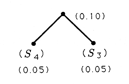
In the late 1950s, David Huffman discovered an algorithm for designing variable-length codes that minimize the average number of bits/symbol. Huffman's algorithm uses a principle of optimality that says, “the optimal code for \(M\) letters has imbedded in it the optimal code for the \(M-1\) letters that result from aggregating the two least likely symbols.” When this principle is iterated, then we have an algorithm for generating the binary tree for a Huffman code:
- label all symbols as “children”;
- “twin” the two least probable children and give the twin the sum of the probabilities:
- (regard the twin as a child; and
- repeat steps (ii) and (iii) until all children are accounted for.
This tree is now labeled with 1's and 0's to obtain the Huffman code. The labeling procedure is to label each right branch with a 1 and each left branch with a 0. The procedure for laying out symbols and constructing Huffman trees and codes is illustrated in the following examples.
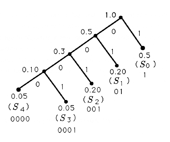
Consider the source statistics
\(\begin{array}{cccccc}
\text { Symbol } & S_{0} & S_{1} & S_{2} & S_{3} & S_{4} \\
\text { Probability } & 0.5 & 0.2 & 0.2 & 0.05 & 0.05
\end{array}\)
for which the Huffman algorithm produces the following binary tree and its corresponding code:
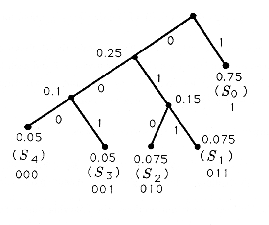
The Huffman code for the source statistics
\(\begin{array}{cccccc}
\text { Symbol } & S_{0} & S_{1} & S_{2} & S_{3} & S_{4} \\
\text { Probability } & 0.75 & 0.075 & 0.075 & 0.05 & 0.05
\end{array}\)
is illustrated next:
Generate binary trees and Huffman codes for the following source statistics:
\(\begin{array}{ccccccccc}
\text { Symbol } & S_{0} & S_{1} & S_{2} & S_{3} & S_{4} & S_{5} & S_{6} & S_{7} \\
\text { Probability1 } & 0.20 & 0.20 & 0.15 & 0.15 & 0.1 & 0.1 & 0.05 & 0.05 \\
\text { Probability2 } & 0.3 & 0.25 & 0.1 & 0.1 & 0.075 & 0.075 & 0.05 & 0.05
\end{array}\)
Coding a FAX Machine
Symbols can arise in unusual ways and be defined quite arbitrarily. To illustrate this point, we consider the design of a hypothetical FAX machine. For our design we will assume that a laser scanner reads a page of black and white text or pictures, producing a high voltage for a black spot and a low voltage for a white spot. We will also assume that the laser scanner resolves the page at 1024 lines, with 1024 spots/line. This means that each page is represented by a two-dimensional array, or matrix, of pixels (picture elements), each pixel being 1 or 0. If we simply transmitted these l's and O′s, then we would need 1024×1024=1,059,576 bits. If these were transmitted over a 9600 baud phone line, then it would take almost 2 minutes to transmit the FAX. This is a long time.
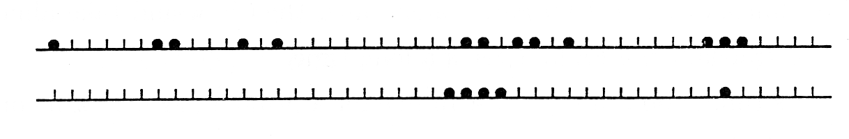
Let's think about a typical scan line for a printed page. It will contain long runs of 0's, corresponding to long runs of white, interrupted by short bursts of l's, corresponding to short runs of black where the scanner encounters a line or a part of a letter. So why not try to define a symbol to be “a run of \(k\) 0's" and code these runs? The resulting code is called a “run length code.” Let's define eight symbols, corresponding to run lengths from 0 to 7 (a run length of 0 is a 1):
\(\begin{aligned}
&S_{0}=\text { run length of } 0 \text { zeros }(a 1) \\
&S_{1}=\quad \text { run length of } 1 \text { zero } \\
&\vdots \\
&S_{7}=\text { run length of } 7 \text { zeros. }
\end{aligned}\)
If we simply used a simple three-bit binary code for these eight symbols, then for each scan line we would generate anywhere from 3×1024 bits (for a scan line consisting of all 1's) to 3 × 1024/7 \(\cong\) 400 bits (for a scan line consisting of all 0's). But what if we ran an experiment to determine the relative frequency of the run lengths \(S_0\) through \(S_7\) and used a Huffman code to “run length encode” the run lengths? The following problem explores this possibility and produces an efficient FAX code.
An experiment conducted on FAXed documents produces the following statistics for run lengths of white ranging from 0 to 7:
\(\begin{array}{ccccccccc}
\text { Symbol } & S_{0} & S_{1} & S_{2} & S_{3} & S_{4} & S_{5} & S_{6} & S_{7} \\
\text { Probability } & 0.01 & 0.06 & 0.1 & 0.1 & 0.2 & 0.15 & 0.15 & 0.2
\end{array}\)
These statistics indicate that only 1% of a typical page is black. Construct the Huffman code for this source. Use your Huffman code to code and decode these scan lines: