Engineering LibreTexts

8.10: Editing Files and Creating Functions (Macintosh)

  • Page ID
    10163
  • \( \newcommand{\vecs}[1]{\overset { \scriptstyle \rightharpoonup} {\mathbf{#1}} } \)

    \( \newcommand{\vecd}[1]{\overset{-\!-\!\rightharpoonup}{\vphantom{a}\smash {#1}}} \)

    \( \newcommand{\id}{\mathrm{id}}\) \( \newcommand{\Span}{\mathrm{span}}\)

    ( \newcommand{\kernel}{\mathrm{null}\,}\) \( \newcommand{\range}{\mathrm{range}\,}\)

    \( \newcommand{\RealPart}{\mathrm{Re}}\) \( \newcommand{\ImaginaryPart}{\mathrm{Im}}\)

    \( \newcommand{\Argument}{\mathrm{Arg}}\) \( \newcommand{\norm}[1]{\| #1 \|}\)

    \( \newcommand{\inner}[2]{\langle #1, #2 \rangle}\)

    \( \newcommand{\Span}{\mathrm{span}}\)

    \( \newcommand{\id}{\mathrm{id}}\)

    \( \newcommand{\Span}{\mathrm{span}}\)

    \( \newcommand{\kernel}{\mathrm{null}\,}\)

    \( \newcommand{\range}{\mathrm{range}\,}\)

    \( \newcommand{\RealPart}{\mathrm{Re}}\)

    \( \newcommand{\ImaginaryPart}{\mathrm{Im}}\)

    \( \newcommand{\Argument}{\mathrm{Arg}}\)

    \( \newcommand{\norm}[1]{\| #1 \|}\)

    \( \newcommand{\inner}[2]{\langle #1, #2 \rangle}\)

    \( \newcommand{\Span}{\mathrm{span}}\) \( \newcommand{\AA}{\unicode[.8,0]{x212B}}\)

    \( \newcommand{\vectorA}[1]{\vec{#1}}      % arrow\)

    \( \newcommand{\vectorAt}[1]{\vec{\text{#1}}}      % arrow\)

    \( \newcommand{\vectorB}[1]{\overset { \scriptstyle \rightharpoonup} {\mathbf{#1}} } \)

    \( \newcommand{\vectorC}[1]{\textbf{#1}} \)

    \( \newcommand{\vectorD}[1]{\overrightarrow{#1}} \)

    \( \newcommand{\vectorDt}[1]{\overrightarrow{\text{#1}}} \)

    \( \newcommand{\vectE}[1]{\overset{-\!-\!\rightharpoonup}{\vphantom{a}\smash{\mathbf {#1}}}} \)

    \( \newcommand{\vecs}[1]{\overset { \scriptstyle \rightharpoonup} {\mathbf{#1}} } \)

    \( \newcommand{\vecd}[1]{\overset{-\!-\!\rightharpoonup}{\vphantom{a}\smash {#1}}} \)

    \(\newcommand{\avec}{\mathbf a}\) \(\newcommand{\bvec}{\mathbf b}\) \(\newcommand{\cvec}{\mathbf c}\) \(\newcommand{\dvec}{\mathbf d}\) \(\newcommand{\dtil}{\widetilde{\mathbf d}}\) \(\newcommand{\evec}{\mathbf e}\) \(\newcommand{\fvec}{\mathbf f}\) \(\newcommand{\nvec}{\mathbf n}\) \(\newcommand{\pvec}{\mathbf p}\) \(\newcommand{\qvec}{\mathbf q}\) \(\newcommand{\svec}{\mathbf s}\) \(\newcommand{\tvec}{\mathbf t}\) \(\newcommand{\uvec}{\mathbf u}\) \(\newcommand{\vvec}{\mathbf v}\) \(\newcommand{\wvec}{\mathbf w}\) \(\newcommand{\xvec}{\mathbf x}\) \(\newcommand{\yvec}{\mathbf y}\) \(\newcommand{\zvec}{\mathbf z}\) \(\newcommand{\rvec}{\mathbf r}\) \(\newcommand{\mvec}{\mathbf m}\) \(\newcommand{\zerovec}{\mathbf 0}\) \(\newcommand{\onevec}{\mathbf 1}\) \(\newcommand{\real}{\mathbb R}\) \(\newcommand{\twovec}[2]{\left[\begin{array}{r}#1 \\ #2 \end{array}\right]}\) \(\newcommand{\ctwovec}[2]{\left[\begin{array}{c}#1 \\ #2 \end{array}\right]}\) \(\newcommand{\threevec}[3]{\left[\begin{array}{r}#1 \\ #2 \\ #3 \end{array}\right]}\) \(\newcommand{\cthreevec}[3]{\left[\begin{array}{c}#1 \\ #2 \\ #3 \end{array}\right]}\) \(\newcommand{\fourvec}[4]{\left[\begin{array}{r}#1 \\ #2 \\ #3 \\ #4 \end{array}\right]}\) \(\newcommand{\cfourvec}[4]{\left[\begin{array}{c}#1 \\ #2 \\ #3 \\ #4 \end{array}\right]}\) \(\newcommand{\fivevec}[5]{\left[\begin{array}{r}#1 \\ #2 \\ #3 \\ #4 \\ #5 \\ \end{array}\right]}\) \(\newcommand{\cfivevec}[5]{\left[\begin{array}{c}#1 \\ #2 \\ #3 \\ #4 \\ #5 \\ \end{array}\right]}\) \(\newcommand{\mattwo}[4]{\left[\begin{array}{rr}#1 \amp #2 \\ #3 \amp #4 \\ \end{array}\right]}\) \(\newcommand{\laspan}[1]{\text{Span}\{#1\}}\) \(\newcommand{\bcal}{\cal B}\) \(\newcommand{\ccal}{\cal C}\) \(\newcommand{\scal}{\cal S}\) \(\newcommand{\wcal}{\cal W}\) \(\newcommand{\ecal}{\cal E}\) \(\newcommand{\coords}[2]{\left\{#1\right\}_{#2}}\) \(\newcommand{\gray}[1]{\color{gray}{#1}}\) \(\newcommand{\lgray}[1]{\color{lightgray}{#1}}\) \(\newcommand{\rank}{\operatorname{rank}}\) \(\newcommand{\row}{\text{Row}}\) \(\newcommand{\col}{\text{Col}}\) \(\renewcommand{\row}{\text{Row}}\) \(\newcommand{\nul}{\text{Nul}}\) \(\newcommand{\var}{\text{Var}}\) \(\newcommand{\corr}{\text{corr}}\) \(\newcommand{\len}[1]{\left|#1\right|}\) \(\newcommand{\bbar}{\overline{\bvec}}\) \(\newcommand{\bhat}{\widehat{\bvec}}\) \(\newcommand{\bperp}{\bvec^\perp}\) \(\newcommand{\xhat}{\widehat{\xvec}}\) \(\newcommand{\vhat}{\widehat{\vvec}}\) \(\newcommand{\uhat}{\widehat{\uvec}}\) \(\newcommand{\what}{\widehat{\wvec}}\) \(\newcommand{\Sighat}{\widehat{\Sigma}}\) \(\newcommand{\lt}{<}\) \(\newcommand{\gt}{>}\) \(\newcommand{\amp}{&}\) \(\definecolor{fillinmathshade}{gray}{0.9}\)

    If you quit MATLAB now, all the commands you have typed will be lost. This is where the Edit window is useful. If you choose new from the File menu, a new window appears with the title Edit 1: Untitled. In this window, you should type in all the commands you would like MATLAB to execute at once. When you are finished typing, you may save the file by choosing save or save as in the file menu and by entering a name for the file. If the edit window is active (that is, if it appears in front), then choose save and go from the file menu to save the file and execute it. If the command window is active, then you can execute the file by entering its name.

    Editing Files

    To test your understanding of file editing, enter the following commands in a file named myfile:

    clear, clg                      %Clear variables and graphics
    j=sqrt(-1);                     %To be sure
    z1=1+.5*j,z2=2+1.5*j            %Enter variables
    z3=z1+z2,z4=z1*z2               %Compute sum and product
    axis([0 4 0 4]),                %First plot
      axis('square'),plot(z1,'o')
    hold on                         %Allow overplot
    plot(z2,'o'),plot(z3,'+'),      %Other plots
        plot(z4,'*')
    hold off

    You do not have to type the % sign and the text that follows it. These are simply comments in a file. They are ignored by the MATLAB interpreter. You should, however, make a habit of adding comments (preceded by %) to your file if you want to be able to understand programs that have been written long ago.

    Do not forget to save your file. Such a file is called a script file. It contains MATLAB commands that could have been entered one by one in the command window. You have three ways to execute a script file:

    1. with the edit window active, choose save and go from the file menu;
    2. with the command window active, enter the file name; or
    3. with the command window active, choose run script... from the M-file menu. In this case, a menu pops up to ask you which file you want to execute.

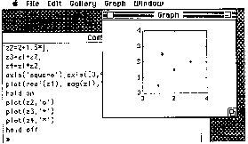
    Try each of these three methods in order to get used to their differences. Figure 1 shows the plot that you should get.

    Creating Functions

    MATLAB puts many commands at your disposal, and you just have to enter their names (with or without arguments) to execute them. Some commands are built in to MATLAB, and others are contained in files to which you have access (not to modify them, but to see how things are done). You can try to display the contents of a command file in the command window by entering the command type filename. Enter type plot. You should get the message

    ??? Built-in function.
    filesfig1.png
    Figure \(\PageIndex{1}\): A Typical Graph (©Apple Computer, Inc., used with permission.)

    This means that the command plot is a build-in function and thus cannot be typed by the user (it is compiled with the program). Similarly, try to type the function file containing the command sinh by entering the command type sinh. You should get

    function y=sinh(x)
    %SINH SINH(X) is the hyperbolic sine of the elements of X.
    y=(exp(x)-exp(-x))/2;

    This is a typical example of a function file. It differs from a script file by the fact that the first line contains the word function. What it does is make the command y = sinh(x) equivalent to the command y=(exp(x)-exp(-x))/2 . The variable x is the input argument (there could be more than one), and \(y\) is the output argument (there also could be more than one). The second line contains comments about the function and its arguments. They can spread to several lines. Display them by typing the command help sinh. The third line contains the actual function commands (there could also be several lines).

    As an exercise, enter the function perp(x):

    function y=perp(x)
    %PERP PERP(X) is a complex value perpendicular to X.
    j=sqrt(-1);
    y=j*real(x)-imag(x);

    Evaluate perp on various complex numbers. Replace the last line by y = x*j;. Do you get the same result? Why?

    Note that local variables are just that–local. Only the input and output arguments are kept in memory after the function is called and executed. For more on functions and multiple arguments, see the MATLAB manual. In the previous example, the variable \(j\) is local. If, before using the function perp, you use the same variable \(j\), its contents will not be affected by the command perp(z). Verify this.

    Normally, while a file (script or function) is executed, the commands are not displayed on the command window. Just the results are displayed. The command echo allows you to view all the instructions. This is useful for debugging and demonstrations. It is turned off by typing echo off.


    This page titled 8.10: Editing Files and Creating Functions (Macintosh) is shared under a CC BY 3.0 license and was authored, remixed, and/or curated by Louis Scharf (OpenStax CNX) via source content that was edited to the style and standards of the LibreTexts platform.