
4.5: Fourier Series Approximation of Signals
- Page ID
- 1617

- Fourier series approximations.
It is interesting to consider the sequence of signals that we obtain as we incorporate more terms into the Fourier series approximation of the half-wave rectified sine wave. Define sK(t) to be the signal containing K+1 Fourier terms.
\[s_{K}(t)=a_{0}+\sum_{k=1}^{K}a_{k}\cos \left ( \frac{2\pi kt}{T} \right )+ \sum_{k=1}^{K}b_{k}\sin \left ( \frac{2\pi kt}{T} \right ) \nonumber \]
Figure 4.5.1 below shows how this sequence of signals portrays the signal more accurately as more terms are added.
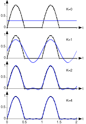
The index indicates the multiple of the fundamental frequency at which the signal has energy. The cumulative effect of adding terms to the Fourier series for the half-wave rectified sine wave is shown in the bottom portion. The dashed line is the actual signal, with the solid line showing the finite series approximation to the indicated number of terms, K+1.
We need to assess quantitatively the accuracy of the Fourier series approximation so that we can judge how rapidly the series approaches the signal. When we use a
\[\varepsilon _{K}(t)=\sum_{k=K+1}^{\infty }a_{k}\cos \left ( \frac{2\pi kt}{T} \right )+ \sum_{k=K+1}^{\infty }b_{k}\sin \left ( \frac{2\pi kt}{T} \right ) \nonumber \]
To find the rms error, we must square this expression and integrate it over a period. Again, the integral of most cross-terms is zero, leaving
\[rms(\varepsilon _{K})=\sqrt{\frac{1}{2}\sum_{k=K+1}^{\infty }a_{k}^{2}+b_{k}^{2}} \nonumber \]
Figure 4.5.2 shows how the error in the Fourier series for the half-wave rectified sinusoid decreases as more terms are incorporated. In particular, the use of four terms, as shown in the bottom plot of Figure 4.5.1 has a rms error (relative to the rms value of the signal) of about 3%. The Fourier series in this case converges quickly to the signal.
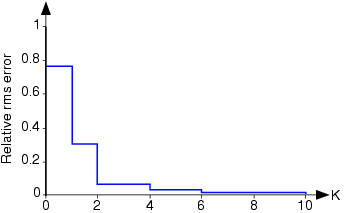
The rms error calculated according to the equation above is shown as a function of the number of terms in the series for the half-wave rectified sinusoid. The error has been normalized by the rms value of the signal.
We can look at Figure 4.5.3 to see the power spectrum and the rms approximation error for the square wave.
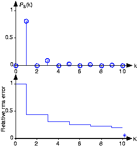
Because the Fourier coefficients decay more slowly here than for the half-wave rectified sinusoid, the rms error is not decreasing quickly. Said another way, the square-wave's spectrum contains more power at higher frequencies than does the half-wave-rectified sinusoid. This difference between the two Fourier series results because the half-wave rectified sinusoid's Fourier coefficients are proportional to 1/k2 while those of the square wave are proportional to 1/k. If fact, after 99 terms of the square wave's approximation, the error is bigger than 10 terms of the approximation for the half-wave rectified sinusoid. Mathematicians have shown that no signal has an rms approximation error that decays more slowly than it does for the square wave.
Calculate the harmonic distortion for the square wave.
Solution
Total harmonic distortion in the square wave is:
\[1-\frac{1}{2}(\frac{4}{\pi })^{2}=20\% \nonumber \]
More than just decaying slowly, Fourier series approximation shown in Figure 4.5.4 exhibits interesting behavior.
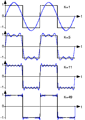
Although the square wave's Fourier series requires more terms for a given representation accuracy, when comparing plots it is not clear that the two are equal. Does the Fourier series really equal the square wave at all values of
Consider this mathematical question intuitively: Can a discontinuous function, like the square wave, be expressed as a sum, even an infinite one, of continuous signals? One should at least be suspicious, and in fact, it can't be thus expressed. This issue brought Fourier much criticism from the French Academy of Science (Laplace, Lagrange, Monge and LaCroix comprised the review committee) for several years after its presentation on 1807. It was not resolved for almost a century, and its resolution is interesting and important to understand from a practical viewpoint.
The extraneous peaks in the square wave's Fourier series never disappear; they are termed Gibb's phenomenon after the American physicist Josiah Willard Gibbs. They occur whenever the signal is discontinuous, and will always be present whenever the signal has jumps.
Let's return to the question of equality; how can the equal sign in the definition of the Fourier series be justified? The partial answer is that pointwise—each and every value of t—equality is not guaranteed. However, mathematicians later in the nineteenth century showed that the rms error of the Fourier series was always zero.
\[\lim_{k \to\infty }rms(\varepsilon _{K})=0 \nonumber \]
What this means is that the error between a signal and its Fourier series approximation may not be zero, but that its rms value will be zero! It is through the eyes of the rms value that we redefine equality: The usual definition of equality is called pointwise equality: Two signals s1(t), s2(t) are said to be equal pointwise if:
\[s_{1}(t)=s_{2}(t) \nonumber \]
for all values of t. A new definition of equality is mean-square equality: Two signals are said to be equal in the mean square if:
\[rms(s_{1}-s_{2})=0 \nonumber \]
For Fourier series, Gibb's phenomenon peaks have finite height and zero width. The error differs from zero only at isolated points—whenever the periodic signal contains discontinuities—and equals about 9% of the size of the discontinuity. The value of a function at a finite set of points does not affect its integral. This effect underlies the reason why defining the value of a discontinuous function, like we refrained from doing in defining the step function, at its discontinuity is meaningless. Whatever you pick for a value has no practical relevance for either the signal's spectrum or for how a system responds to the signal. The Fourier series value "at" the discontinuity is the average of the values on either side of the jump.