8.8: Ideal Impulse Response Versus Real Response of Systems

Section 8.5 shows that, for a 1^st order system subjected to excitation by an ideal impulse function, the post-impulse initial value at \(t=0^{+}\) of output \(x(t)\) differs from the pre-impulse initial value at \(t=0^{-}\). Let us now investigate the initial values in \(x(t)\) and \(\dot{x}(t)\) that are associated with the 2^nd order system of Section 8.7. The output itself is given by Equation 8.7.3: \(x(t)=\left(\omega_{n} I_{U}+\dot{x}_{0} / \omega_{n}\right) \sin \omega_{n} t+x_{0} \cos \omega_{n} t, t \geq 0^{+}\), \(t \geq 0^{+}\). Evaluating this equation at \(t=0^{+}\) shows that the post-impulse value is \(x\left(0^{+}\right)=x_{0}\); this is exactly the same value as the given initial value at \(t=0^-\), so there is no discontinuous change in the initial value of \(x(t)\) itself for the 2^nd order system. Differentiating Equation 8.7.3 gives the “velocity” function:

\[\dot{x}(t)=\left(\omega_{n}^{2} I_{U}+\dot{x}_{0}\right) \cos \omega_{n} t-\omega_{n} x_{0} \sin \omega_{n} t, t \geq 0^{+}\label{eqn:8.29} \]

Evaluating Equation \(\ref{eqn:8.29}\) at \(t=0^{+}\) gives

\[\dot{x}\left(0^{+}\right)=\omega_{n}^{2} I_{U}+\dot{x}_{0} \neq \dot{x}_{0}=\dot{x}\left(0^{-}\right)\label{eqn:8.30} \]

Thus, for the 2^nd order system, there is a discontinuous change in the initial value of the "velocity" function.

The discontinuous changes that we observe in initial values for both 1^st and 2^nd order systems violate physical laws governing real systems, so ideal impulse response solutions appear to be defective and perhaps not applicable to real systems. The reason for this defectiveness is the ideal, not real, nature of the Dirac delta function \(\delta(t)\). In physical reality, there is no such thing as a pulse of infinitely short duration and infinitely great magnitude; so \(\delta(t)\) and \(I_{U} \delta(t)\) are mathematical functions that do not represent exactly any real physical quantities.

However, the ideal impulse responses that we find can still be useful in applications to real systems, because the ideal impulse function \(I_{U} \delta(t)\) can approximate the effect of a real, time-limited pulse that has the same impulse magnitude, \(I_{U}\); therefore, the ideal impulse response can approximate the actual physical response. Why would we use the approximate ideal impulse response rather than just determining the more precise response solution based upon the actual pulse? We would do this because it is always much easier to derive and compute the ideal impulse response than the actual pulse response; moreover, the equation for the ideal impulse response is always simpler and more amenable to practical purposes (such as system identification, a form of which is discussed in Section 9.9) than the equation(s) for the actual pulse response.

When is ideal impulse response a good approximation of real pulse response, and when is it not? It depends on the duration \(t_d\) of the actual input pulse relative to the shortest characteristic time \(T_c\) of the system that is being analyzed. The characteristic time is defined loosely as the time interval required for system response to change substantially. The system characteristic times that we know from previous chapters are time constant \(\tau_{1}\) for a 1^st order system and about one quarter of a natural period \(T_{n}\) for a 2^nd order system. If \(t_d\) is brief relative to the system characteristic time, \(t_{d}<<T_{c}\), then the ideal impulse response [Equation 8.5.4 for a standard stable 1^st order system, Equation 8.7.3 for a standard undamped 2^nd order system, other equations for other types of systems] will be a good approximation to the actual pulse response; on the other hand, if \(t_d\) is on the order of or greater than the system characteristic time, \(\mathrm{O}\left(t_{d}\right) \geq \mathrm{O}\left(T_{c}\right)\), then the ideal impulse response would be a poor approximation, and we should solve for the response using the actual physical pulse. There is no hard and fast rule as to how small the ratio \(t_{d} / T_{c}\) should be to justify use of the ideal impulse response solution.

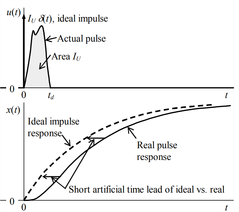
In what manner would ideal impulse response differ from the actual pulse response? Let us consider, for example, an undamped 2^nd order system with zero ICs. Suppose that the duration of the actual pulse satisfies \(t_{d}<<1 / 4 T_{n}\), so that, according to the discussion above, the ideal impulse response should be a good approximation to the actual response. But we already know from Equation \(\ref{eqn:8.30}\) that the initial velocity of the ideal impulse response will be wrong, with value \(\omega_{n}^{2} I_{U}\) when it ought to be zero. How will the remainder of the ideal impulse response compare with the actual response? Figure \(\PageIndex{1}\) depicts conceptually the nature of both ideal impulse response and the comparable real response for a 2^nd order system during the initial portion of response. The real response shows the correct initial zero slope, \(\dot{x}_{0}=0\). For a brief period after \(t = 0\), the slope of real response increases rapidly until both the response \(x\) and the slope \(\dot{x}\) essentially match the comparable values of the ideal response, but with a short time lag relative to the ideal response. In other words, the ideal response has a short, artificial time lead relative to the real response. After the pulse ends, \(t_{d}<t\), the real response is essentially identical to the ideal response, but the ideal response maintains the same artificial time lead for all of the remaining dynamic response. If the pulse duration is very short relative to the system quarter-period, then the artificial time lead will be very small, perhaps not even detectable on a graph of the response. In this case, ideal impulse response will clearly be an excellent approximation to the actual response, and the ideal impulse response will be much easier to derive and compute the actual response.

Figure \(\PageIndex{1}\): Conceptual ideal impulse response and real pulse response for an undamped 2^nd order system

Note that the previous paragraph applies specifically for a 2^nd order system, but not necessarily for other system types. In particular, for a 1^st order system, the differences between a real pulse response and the approximating ideal impulse response have a different character (see, for example, homework Problem 8.5).