8.10: The Convolution Integral as a Superposition of Ideal Impulse Responses

Last updated
Save as PDF

Page ID: 8045

\( \newcommand{\vecs}[1]{\overset { \scriptstyle \rightharpoonup} {\mathbf{#1}} } \) \( \newcommand{\vecd}[1]{\overset{-\!-\!\rightharpoonup}{\vphantom{a}\smash {#1}}} \)\(\newcommand{\id}{\mathrm{id}}\) \( \newcommand{\Span}{\mathrm{span}}\) \( \newcommand{\kernel}{\mathrm{null}\,}\) \( \newcommand{\range}{\mathrm{range}\,}\) \( \newcommand{\RealPart}{\mathrm{Re}}\) \( \newcommand{\ImaginaryPart}{\mathrm{Im}}\) \( \newcommand{\Argument}{\mathrm{Arg}}\) \( \newcommand{\norm}[1]{\| #1 \|}\) \( \newcommand{\inner}[2]{\langle #1, #2 \rangle}\) \( \newcommand{\Span}{\mathrm{span}}\) \(\newcommand{\id}{\mathrm{id}}\) \( \newcommand{\Span}{\mathrm{span}}\) \( \newcommand{\kernel}{\mathrm{null}\,}\) \( \newcommand{\range}{\mathrm{range}\,}\) \( \newcommand{\RealPart}{\mathrm{Re}}\) \( \newcommand{\ImaginaryPart}{\mathrm{Im}}\) \( \newcommand{\Argument}{\mathrm{Arg}}\) \( \newcommand{\norm}[1]{\| #1 \|}\) \( \newcommand{\inner}[2]{\langle #1, #2 \rangle}\) \( \newcommand{\Span}{\mathrm{span}}\)\(\newcommand{\AA}{\unicode[.8,0]{x212B}}\)

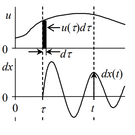
Suppose that an LTI system has zero ICs and that the input is an arbitrary physically realistic function, \(u(t)\) for \(t>0\). Let us apply directly the principle of superposition to derive an equation for response \(x(t)\) at some arbitrary instant of time \(t > 0\). At any instant \(\tau\) less than \(t\), \(0<\tau<t\), the input \(u(\tau)\) imposes onto the system a differentially small impulse of magnitude \(d I_{U}=u(\tau) d \tau\), as is indicated conceptually on the figure below.Then the differentially small response at time \(t>\tau\) due to this impulse at \(\tau\) is \(d x(t)=d I_{U} \times h(t-\tau)=u(\tau) h(t-\tau) d \tau\), in which \(h(t-\tau)\) is the IRF due to a unit impulse acting at instant \(\tau\). Because this system is linear, we can express the total response as the superposition of responses due to all separate inputs, as is stated in Section 1.2. In this case, there are an infinite number of instants \(\tau\) between time zero and time \(t\), so the superposition, or summation, becomes a definite integral:

\[\left.x(t)\right|_{I C s=0}=\int_{\tau=0}^{\tau=t} d x(t)=\int_{\tau=0}^{\tau=t} u(\tau) h(t-\tau) d \tau\label{eqn:8.41} \]

Equations such as Equation \(\ref{eqn:8.41}\) and its versions for specific systems [with explicit functions for \(h(t-\tau)\)] are often called Duhamel integrals (after Jean-Marie Duhamel, 1797-1872, rench mathematician and physicist), especially in the literature of structural dynamics (e.g., C F raig, 1981, p. 124).

Equation (8-41) is general, valid for any LTI system. To see a specific application, let us re-visit the standard undamped 2^nd order system. With \(I_{U}=1\), Equation 8.7.3 gives the IRF as \(h(t)=\omega_{n} \sin \omega_{n} t\), so Equation \(\ref{eqn:8.41}\) becomes

\[\left.x(t)\right|_{I C s=0}=\omega_{n} \int_{\tau=0}^{\tau=t} u(\tau) \sin \omega_{n}(t-\tau) d \tau\label{eqn:8.42} \]

Equation \(\ref{eqn:8.42}\) is the Duhamel integral response solution for the standard undamped 2^nd order system, and it is identical to convolution integral response solution Equation 7.2.5 with zero ICs. Recall that Equation 7.2.5 was derived mostly from the mathematics of convolution integrals and transforms in Chapter 6. On the other hand, the derivation of Equation \(\ref{eqn:8.42}\) above is primarily physical, based upon the IRF and the principle of superposition for linear systems.