9.8: Step-Response Specifications for Underdamped Systems

Engineering systems are often designed so that the time history of an output quantity will mimic as closely as possible the time history of the input quantity. An example, with reference to Section 3.5, is the aileron-induced rolling of an airplane, for which the original input is the control wheel angle set manually (“commanded”) by the pilot, and the ultimate output is the airplane roll rate. Another example is the modern automobile; we usually describe a car as being “responsive” if the steering (or the acceleration, or the braking) mimics quickly and precisely the driver’s commands set by hand or foot.

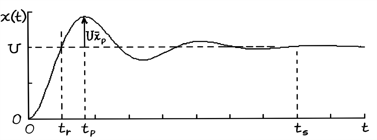
Step response of a system is often used for measuring and quantifying dynamic “responsiveness.” Ideally, step response would mimic exactly the step input, but system characteristics such as inertia and damping prevent such instantaneous response. The degree to which step response fails to mimic step input is quantified in the following four step-response specifications: rise time, \(t_{r}\); peak time, \(t_{p}\), maximum overshoot ratio, \(\bar{x}_{p}\), and settling time, \(t_{s}\). These step-response quantities are illustrated on Figure 9.6 on the next page. They are called “specifications” or “specs” because it is common in the beginning of a project to specify them as design targets; later, these step-response quantities are measured experimentally on prototype and/or production test articles.

Figure \(\PageIndex{1}\): Step-response specifications of an underdamped system

For underdamped 2^nd order systems, we can apply step-response solution Equation 9.6.5 and impulse-response solution Equation 9.7.2 to derive specific equations for the step-response specifications:

• From Figure \(\PageIndex{1}\), we evaluate Equation 9.6.5 at \(t=t_{r}\), the first time when \(x(t) = U\):\[x\left(t_{r}\right)=U=U\left[1-e^{-\zeta \omega_{n} t_{r}}\left(\cos \omega_{d} t_{r}+\frac{\zeta \omega_{n}}{\omega_{d}} \sin \omega_{d} t_{r}\right)\right] \Rightarrow \cos \omega_{d} t_{r}+\frac{\zeta \omega_{n}}{\omega_{d}} \sin \omega_{d} t_{r}=0 \nonumber \]\[\Rightarrow \tan \omega_{d} t_{r}=-\frac{\omega_{d}}{\zeta \omega_{n}}=-\frac{\sqrt{1-\zeta^{2}}}{\zeta}=-\frac{1}{\zeta_{s}} \nonumber \]This last equation shows that as \(\zeta \rightarrow 0\) from positive values, then \(\tan \omega_{d} t_{r} \rightarrow-\infty\) from negative values; therefore, \(\omega_{d} t_{r} \rightarrow \frac{1}{2} \pi \times n\) from higher values, where \(n = 1, 5, 9, \dots\); and the first time when \(x(t) = U\) corresponds to \(n = 1\): \(\omega_{d} t_{r} \rightarrow \frac{1}{2} \pi\) from higher values. We can see this in Figure 9.6.1, where \(t_{r}\) is just a bit after \(\frac{1}{2} \pi / \omega_{n}\) (keep in mind that \(\omega_{d} \leq \omega_{n}\)). This leads to the conclusion that the rise time is given by\[t_{r}=\frac{1}{\omega_{d}} \tan ^{-1}\left(\frac{\sqrt{1-\zeta^{2}}}{-\zeta}\right)\label{eqn:9.33} \]In Equation \(\ref{eqn:9.33}\), we take the value of the four-quadrant inverse tangent that is between \(\frac{1}{2} \pi\) and \(\pi\), as shown on the drawing below.

  

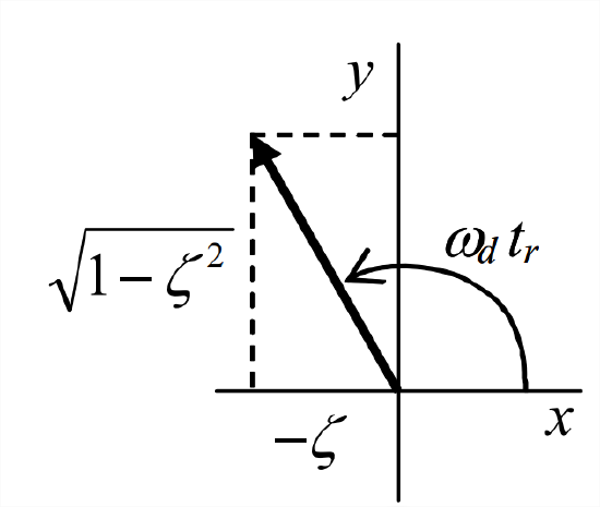
  Figure \(\PageIndex{2}\)

• From Figure \(\PageIndex{1}\), \(t_p\) is the time at which \(x(t)\) is maximum and the first time after \(t = 0\) that \(t= 0\). So we need to differentiate Equation 9.6.5, set it to zero, and solve for \(t_p\) from the resulting equation. From the appearance of Equation 9.6.5, though, that differentiation will be long and tedious. But that drudgery will not be necessary, because a fundamental relationship derived in Section 8.7 will come to our rescue. We identify the unit-step response as Equation 9.6.5 with step magnitude \(U = 1\):\[x_{H}(t)=1 \times\left[1-e^{-\zeta \omega_{n} t}\left(\cos \omega_{d} t+\frac{\zeta \omega_{n}}{\omega_{d}} \sin \omega_{d} t\right)\right]=1-e^{-\zeta \omega_{n} t}\left(\cos \omega_{d} t+\frac{\zeta \omega_{n}}{\omega_{d}} \sin \omega_{d} t\right)\label{eqn:9.34} \]Clearly, \(t_p\) is independent of step magnitude \(U\). Now, Equation 8.6.6 gives the derivative of Equation \(\ref{eqn:9.34}\) as \(d x_{H} / d t=h(t)\), where the IRF \(h(t)\) in this case is Equation 9.7.3. Therefore, the equation leading to that we seek is\[\frac{d x_{H}}{d t}=h(t)=\frac{\omega_{n}^{2}}{\omega_{d}} e^{-\zeta \omega_{n} t} \sin \omega_{d} t=0 \text { at } t=t_{P}\label{Eqn:9.35} \]The required solution of Equation \(\ref{eqn:9.35}\) is the lowest positive value of \(t\) that satisfies \(\sin \omega_{d} t= 0\), which is\[t_{p}=\frac{\pi}{\omega_{d}}\label{eqn:9.36} \]The graphical equivalent of this mathematical derivation of Equation \(\ref{eqn:9.36}\) is evident in an examination of Figures 9.6.1 and 9.7.1, where we can see that both the peak of the step response and the first zero of the ideal impulse response occur at an instant \(t\) just a bit after \(\pi / \omega_{n}\) (recall that \(\omega_{d} \leq \omega_{n}\)).
• From Figure \(\PageIndex{1}\), Equation 9.6.5, and Equation \(\ref{eqn:9.36}\), the maximum overshoot ratio is\[\bar{x}_{p}=\frac{x\left(t_{p}\right)-U}{U}=-e^{-\zeta \omega_{n} t_{p}}\left(\cos \omega_{d} t_{p}+\frac{\zeta \omega_{n}}{\omega_{d}} \sin \omega_{d} t_{p}\right)=-\exp \left(-\zeta \omega_{n} \frac{\pi}{\omega_{d}}\right)\left(\cos \pi+\frac{\zeta \omega_{n}}{\omega_{d}} \sin \pi\right) \nonumber \]\[\Rightarrow \quad \bar{x}_{p}=\exp \left(-\frac{\zeta}{\sqrt{1-\zeta^{2}}} \pi\right) \leq 1, \text { valid for } 0 \leq \zeta<1\label{eqn:9.37} \]So the maximum overshoot ratio is a function only of viscous damping ratio \(\zeta\). Conversely, \(\zeta\) can be determined from a measurement of \(\bar{x}_{p}\) by taking the natural logarithm of Equation \(\ref{eqn:9.37}\):\[\ln \bar{x}_{p}=-\frac{\zeta}{\sqrt{1-\zeta^{2}}} \pi \Rightarrow-\frac{\ln \bar{x}_{p}}{\pi}=\frac{\zeta}{\sqrt{1-\zeta^{2}}} \equiv \zeta_{s}, \text { valid for } 0<\bar{x}_{p} \leq 1\label{eqn:9.38} \]Note the similarity of Equation \(\ref{eqn:9.38}\) to Equation 9.5.3 for the logarithmic decrement. Therefore, we arrive again at Equation 9.5.4, the exact equation giving \(\zeta\) for any overshoot in the range \(0<\bar{x}_{p} \leq 1\): \(\zeta=\zeta_{s} / \sqrt{1+\zeta_{s}^{2}}\), for \(0 \leq \zeta<1\), now with \(\zeta_{s}=-\ln \bar{x}_{p} / \pi\).

  If damping is small such that \(\sqrt{1-\zeta^{2}} \approx 1\), i.e., \(0 \leq \zeta \leq 0.2\), then Equations \(\ref{eqn:9.37}\) and \(\ref{eqn:9.38}\) are approximated as:\[\bar{x}_{p} \approx e^{-\zeta \pi} \quad \text { and } \quad \zeta \approx-\frac{\ln \bar{x}_{p}}{\pi} \quad \text { valid for } 0 \leq \zeta \leq 0.2 \text { and } 0.534 \leq \bar{x}_{p} \leq 1\label{eqn:9.39} \]

• This specification is defined as the time required for response \(x(t)\) to settle to within \(\pm 2%\) of the final steady-state (pseudo-static) value, \(U\). For this underdamped 2^nd order system, the time constant of the exponential envelope is Equation 9.4.3, \(\tau_{2} \equiv 1 / \zeta \omega_{n}\). From Chapter 3, we have \(1-e^{-4}=0.982\) (see Figure 3.4.2), so the settling time is defined as \[t_{s}=4 \tau_{2} \equiv \frac{4}{\zeta \omega_{n}}\label{eqn:9.40} \]

  It is appropriate here to evaluate the variation in step response of a standard 2^nd order system as damping varies. Figure \(\PageIndex{3}\) on the next page displays 2^nd order step responses for a range of viscous damping ratios \(\zeta\). [The response curves of Figure \(\PageIndex{3}\) are calculated as follows: for underdamping, \(0 \leq \zeta<1\), from Equation 9.6.5; for critical damping, \(\zeta=1\), from the result of homework Problem 9.11; for overdamping, \(\zeta=1.2\), from the result of homework Problem 9.16. The time reference is undamped natural period \(T_{n}=2 \pi / \omega_{n}\).] As engineers designing a system, we might wish to design into the system a quantity of damping \(\zeta\) that makes the time history of an output quantity mimic as closely as possible the time history of the input quantity. This means, in the context of step response, we would want both to make rise time as fast as possible and to minimize overshoot. However, Figure \(\PageIndex{3}\) shows that we cannot simultaneously do both for a standard 2^nd order system: rise time is fastest for small \(\zeta\), but overshoot is minimized or eliminated with larger \(\zeta\). Therefore, we would have to compromise and select a value of \(\zeta\) that produces practically acceptable values of both rise time and overshoot, even though neither response parameter would be the best possible. Observe from Figure \(\PageIndex{3}\) that overshoot exists only for underdamping.

  

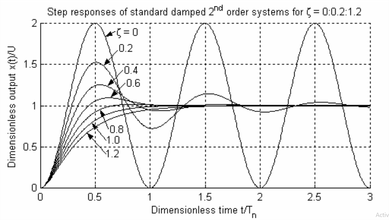
  Figure \(\PageIndex{3}\): Step responses of standard 2^nd order systems as viscous damping varies

  The transient response of engineered control systems is very important in practice, so there is more analysis and discussion of subjects such as rise time and overshoot later in the book, beginning in Chapter 14.