
9.11: Chapter 9 Homework
- Page ID
- 8347

\( \newcommand{\vecs}[1]{\overset { \scriptstyle \rightharpoonup} {\mathbf{#1}} } \) \( \newcommand{\vecd}[1]{\overset{-\!-\!\rightharpoonup}{\vphantom{a}\smash {#1}}} \)\(\newcommand{\id}{\mathrm{id}}\) \( \newcommand{\Span}{\mathrm{span}}\) \( \newcommand{\kernel}{\mathrm{null}\,}\) \( \newcommand{\range}{\mathrm{range}\,}\) \( \newcommand{\RealPart}{\mathrm{Re}}\) \( \newcommand{\ImaginaryPart}{\mathrm{Im}}\) \( \newcommand{\Argument}{\mathrm{Arg}}\) \( \newcommand{\norm}[1]{\| #1 \|}\) \( \newcommand{\inner}[2]{\langle #1, #2 \rangle}\) \( \newcommand{\Span}{\mathrm{span}}\) \(\newcommand{\id}{\mathrm{id}}\) \( \newcommand{\Span}{\mathrm{span}}\) \( \newcommand{\kernel}{\mathrm{null}\,}\) \( \newcommand{\range}{\mathrm{range}\,}\) \( \newcommand{\RealPart}{\mathrm{Re}}\) \( \newcommand{\ImaginaryPart}{\mathrm{Im}}\) \( \newcommand{\Argument}{\mathrm{Arg}}\) \( \newcommand{\norm}[1]{\| #1 \|}\) \( \newcommand{\inner}[2]{\langle #1, #2 \rangle}\) \( \newcommand{\Span}{\mathrm{span}}\)\(\newcommand{\AA}{\unicode[.8,0]{x212B}}\)
- In the system drawn below, mass \(m\) is attached to a movable support by viscous dashpot \(c_1\) and spring \(k\), and the mass also slides on a lubricated surface, which causes viscous damping with constant \(c_2\). There are two independent input quantities: The output quantity is displacement \(x(t)\) of the mass. Sketch and label clearly appropriate free-body diagrams, then use your FBD to derive the differential equation of motion for \(x(t)\) in terms of constants \(m\), \(c_1\), \(c_2\) and \(k\), and variable inputs \(x_{i}(t)\) and \(f_{x}(t)\). Your ODE of motion should include some non-standard right-handside dynamics.
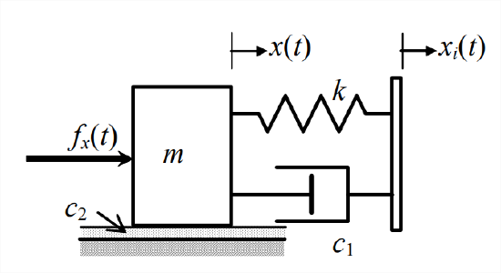
Figure \(\PageIndex{1}\) - support displacement \(x_{i}(t)\) shown (displacement control, e.g., by a cam), which is often called base excitation1, and
- force \(f_{x}(t)\) shown.
- Given, a standard \(m\)-\(c\)-\(k\) system, Figure 9.1.1, with the following parameters: weight of the mass \(W=0.386\) lb, so that \(m=\frac{W}{g}=\frac{0.386 \mathrm{lb}}{386 \mathrm{inch} / \mathrm{s}^{2}}=0.001 \frac{\mathrm{lb}-\mathrm{s}^{2}}{\text { inch }}\); damper viscous constant \(c=1.1 \times 10^{-3}\) lb/inch/s; spring stiffness constant \(k=3.025\) lb/inch.
- Calculate the following quantities, all to at least 3 significant figures: \(\omega_{n}\) in rad/s, \(f_{n}\) in Hz, \(\zeta\), \(\omega_{d}\) in rad/s, \(f_d\) in Hz, and \(T_{d} \equiv 1 / f_{d}\). You may calculate these quantities in MATLAB, if you wish, using the command
format short e. - Given initial conditions \(x(0)=0.5\) inch and \(\dot{x}(0)=35\) inch/s, calculate and graph with MATLAB the free-vibration response due to the ICs over about 20 complete decaying cycles. Since you are multiplying sinusoidal time functions by an exponential time function, it is necessary that you use array multiplication (.*) in MATLAB. Draw grids on your graph and add an appropriate title and appropriate axis labels.
- Sketch by hand the exponential envelope on your graph, then use the grids and/or a graduated straight edge to measure amplitudes of local peaks of the decaying sinusoid. In particular, find (approximately) the quantity \(r_{1 / 2} \equiv\) the number of decaying cycles to decay to half amplitude (not necessarily an integer). Now calculate the dimensionless ratio \(0.110 / r_{1 / 2}\); the value that you calculate should match closely with your previously calculated value of \(\zeta\).
- Calculate the following quantities, all to at least 3 significant figures: \(\omega_{n}\) in rad/s, \(f_{n}\) in Hz, \(\zeta\), \(\omega_{d}\) in rad/s, \(f_d\) in Hz, and \(T_{d} \equiv 1 / f_{d}\). You may calculate these quantities in MATLAB, if you wish, using the command
- The free-vibration response to initial conditions of a standard damped 2nd order system is given by \(x(t)=2.24 e^{-0.300 t} \cos (12.00 t-1.11)\) mm, where \(t\) is in seconds. Calculate
- the damped natural frequency \(f_{d}\) in Hz,
- the damping time constant \(\tau_{2}\) in seconds, and
- the viscous damping ratio \(\zeta\) (use the small-\(\zeta\) approximation). Show your calculations.
- A simple type of vibration testing often used for underdamped mechanical systems, such as the \(m\)-\(c\)-\(k\) system of Figure 9.1.1, is called twang testing (named after the sharp, ringing sound made by plucking a string of a musical instrument; Section 7.6 demonstrates twang testing of a flexible beam): the mass is displaced from its static equilibrium position by amount \(x_{0}\) (with zero initial velocity, \(\dot{x}_{0}=0\)), then it is released. From the record of subsequent transient response, we can calculate directly the damped natural frequency \(f_d\) and the viscous damping ratio \(\zeta\). If we know initially either the mass \(m\) or the stiffness constant \(k\), then we can use the measured \(f_d\) and \(\zeta\) to calculate the other constant and the effective viscous damping constant \(c\). Use Equation 9.4.2 to show that twang test response is \[x(t)=x_{\max } e^{-\zeta \omega_{n} t} \cos \left(\omega_{d} t+\phi\right), \text { for } 0 \leq t \text { and } 0 \leq \zeta<1 \nonumber \] where \(x_{\max }=x_{0} / \sqrt{1-\zeta^{2}}\) and \(\phi=\tan ^{-1}(-\zeta / \sqrt{1-\zeta^{2}})\) For a very lightly damped system, the preferred simple approximation of this twang response is \[x(t) \approx x_{0} e^{-\zeta \omega_{n} t} \cos \left(\omega_{n} t\right), \text { with } \phi \approx 0 \nonumber \] How small must \(\zeta\) be so that phase lag \(\phi\) is so small (say, \(|\phi| \leq 5^{\circ}\)) that it can not be distinguished from zero phase lag, \(\phi \approx 0\)? [NOTE: the measurement resolution on a typical analog graphical record of transient-decay vibration response (for example, from a small oscilloscope screen) is so limited that the resolution of calculated phase is probably only around \(\pm 5^{\circ}\).
- A laboratory mass-damper-spring system was set into motion and then allowed to vibrate freely. The time-history acceleration on the next page was sensed by a lightweight accelerometer attached to the mass. The graph was copied from the screen of a digital oscilloscope. Calculate from measurements on a photocopy of the graph the damped natural frequency \(f_d\) (Hz) = \(\omega_{d} / 2 \pi\) and the viscous damping ratio \(\zeta\). In order to obtain reasonably accurate values for \(f_d\) and \(\zeta\), be sure to average over many cycles of the damped sinusoid. To calculate \(\zeta\), first sketch in the exponential envelope. Also, note that the zero level of the acceleration signal is offset from the center horizontal grid line; therefore, peak-to-peak amplitude measurements are more appropriate than zero-to-peak measurements, as well as more accurate. Annotate your measurements on the graph (submit the annotated graph), and show your calculations clearly. From your values for \(f_d\) and \(\zeta\), calculate the undamped natural frequency \(f_n\) (Hz). For a lightly damped system such as this one, is the difference between \(f_d\) and \(f_n\) numerically significant, given the limited precision of the measured quantities?
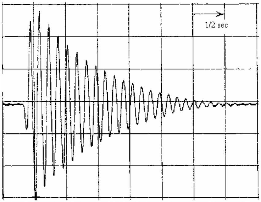
Figure \(\PageIndex{2}\) - A standard \(m\)-\(c\)-\(k\) system is initially at rest. Then an engineer strikes the mass with a soft-tipped hammer that produces a relatively slow half-sine force pulse of amplitude 25 lb and duration 0.1 s [\(f_{x}(t)=25 \mathrm{lb} \times \sin (10 \pi t)\) for \(0 \leq t \leq 0.1\) s]. Both the force pulse \(f_{x}(t)\) and the displacement response \(x(t)\) of the mass are recorded on the graph below. To support the calculations assigned (next page), annotate your measurements on a photocopy of the graph (hand in the annotated graph), and show your calculations clearly.
- Calculate from the \(f_x(t)\) equation the impulse produced by the force. However, you should not use this \(I_F\) in Equation 9.9.3 to determine \(m\). Explain why not.
- Calculate from the graph, with as much accuracy as the data permits, the damped natural frequency \(f_d\) (Hz), and the viscous damping ratio \(\zeta\) of the system.
- The system’s mass \(m\) is known to be 0.0652 lb-s2/inch. Calculate stiffness constant \(k\) and damping constant \(c\).
- A large mass-damper-spring (\(m\)-\(c\)-\(k\)) system is initially at rest. Then a machine imposes upon the mass a slowly varying force in the form of a sawtooth pulse of amplitude 800 N and pulse duration 1.5 s, \(f_{x}(t)=\frac{800 \mathrm{N}}{1.5 \mathrm{s}} \times t\) for \(0 \leq t \leq 1.5\) s. Both the force pulse \(f_{x}(t)\) and the displacement response \(x(t)\) of the mass are recorded on the graph below. The unusual displacement scale “ (mm * 100)” is employed in order to accommodate the ranges of both \(f_{x}(t)\) and \(x(t)\) on the same graph; this scale simply means that the range of displacements on the graph is \(-6.00 \mathrm{mm} \leq x(t) \leq+8.00 \mathrm{mm}\). To support the calculations assigned (next page), annotate your measurements on a photocopy of the graph (hand in the annotated graph), and show your calculations clearly.
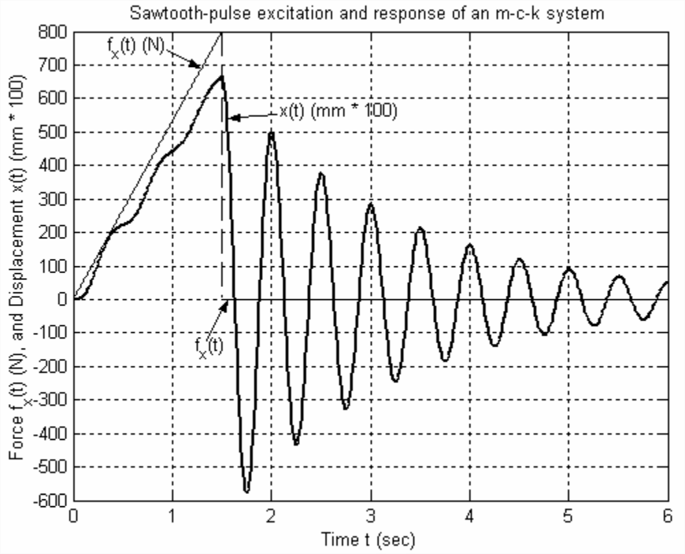
Figure \(\PageIndex{3}\) - Calculate the total impulse \(I_F\) produced by the force. However, you should not use this \(I_F\) in Equation 9.9.3 to determine \(m\). Explain why not.
- Calculate from the graph, with as much accuracy as the data permits, the damped natural frequency \(f_d\) (Hz), and the viscous damping ratio \(\zeta\) of the system.
- The system’s stiffness constant \(k\) is known from static testing to be 120.0 kN/m. Calculate mass \(m\) and damping constant \(c\).
- Find the algebraic/numerical equation for the pseudo-static response \(x_{p s}(t)\) while the pulse is active (\(0 \leq t \leq 1.5\) s), and compare your \(x_{p s}(t)\) with the actual response \(x(t)\) on the graph.
- Consider the mass-damper-spring system shown in the figure below, with: The system is initially at rest (the left-hand figure) in the static equilibrium position for weight \(m_{0} g\). At \(t\) = 0, mass \(m_1\) is gently placed upon \(m_0\) and then released. This imposes an \(m_{1} g\) step force (the weight, due to gravity) onto the system. Note also that mass \(m_1\) changes the system, since the total vibrating mass now will be \(m_{0}+m_{1}\), not just \(m_{0}\). Use Equation 9.6.5 for underdamped 2nd order system step response to write the numerical equation for response \(y(t)\) in inches of combined mass \(m_{0}+m_{1}\) (relative to the static equilibrium position for the weight of \(m_0\) alone, as indicated on the figure). Then use MATLAB to plot the response curve of \(y(t)\) versus \(t\) from \(t\) = 0 until the mass has settled to within at least 2% of its final steady-state position. This means plot to at least four time constants, \(t=4 \tau_{2}\), where \(\tau_{2}=\left(\zeta \omega_{n}\right)^{-1}\). Since you are multiplying sinusoidal time functions by an exponential time function, it is necessary that you use array multiplication (.*) in MATLAB. Provide appropriate grids, titles, and labels on your graph. It is not required, but you can check from your graph that the response has the values of frequency, steady-state (final static, pseudo-static) displacement, and viscous damping ratio that you can calculate from the original data for mass, damping, stiffness, and applied force.
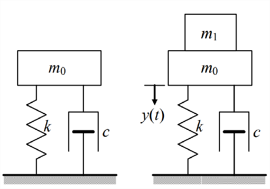
Figure \(\PageIndex{4}\) - \(m_0\) = 10.0 kg, \(c\) = 40.0 N-s/m, \(k\) = 400 N/m, and \(m_1\) = 2.00 kg;
- \(m_{0} g\) = 225 lb, \(c\) = 2.10 lb-s/inch, \(k\) = 30.5 lb/inch, and \(m_{1} g\) = 105 lb.
- For the \(m\)-\(c\)-\(k\) system and step input/response of homework Problem 9.8 [part 9.8.1 or 9.8.2, whichever is assigned], use the equations of Section 9.8 to calculate rise time \(t_r\), peak time \(t_p\), maximum overshoot ratio \(\bar{y}_{p}\), and settling time \(t_s\). These calculations should agree with the comparable results that you can measure from your MATLAB step-response graph for homework Problem 9.8, assuming that your graph is correct.
- Weight \(W_{2}\) = 98.1 N (mass \(m_2\) = 10.0 kg) is suspended by a string from weight \(W_1\) = 196.2 N (mass \(m_1\) = 20.0 kg), which is attached to the ceiling by spring \(k\) and viscous dashpot \(c\), as shown below. The system is in static equilibrium when, at time \(t\) = 0, the string is cut cleanly, dropping \(W_{2}\). (This simulates the release of a bomb from a flexible airplane wing.) Consider the subsequent motion \(x(t)\), \(t \geq 0\), of \(m_1\). With the \(y(t)\) datum shown on the drawing, you can think of this as step-response, with the release of \(W_{2}\) being equivalent to imposing upon \(m_1\) an upward step force equal to \(W_{2}\).
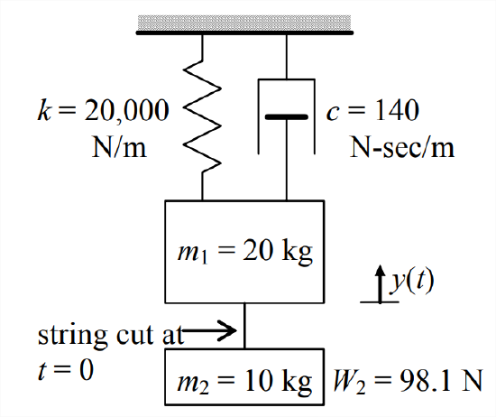
Figure \(\PageIndex{5}\) - Calculate the undamped natural frequency \(f_n\) (Hz), the damping ratio \(\zeta\), the damped natural frequency \(f_d\) (Hz), and the damped period of oscillation \(T_d\) (s).
- Calculate the final (as \(t \rightarrow \infty\)) static value of \(y\) and the settling time \(t_s\) required for the motion to settle within 2% of that final static value.
- Sketch a plot of the response \(y(t)\) versus \(t\) from \(t = 0\) until about \(t = t_s\). Do not carry out extensive calculations; just use the results of parts 9.10.1 and 9.10.2 to sketch an engineer’s back-of-the-envelope type of quick graph that clearly shows the principal features of the response, but is not precise like a computer-generated graph.
- Derive the algebraic equation for step response \(x(t)\) with zero ICs of critically damped 2nd order systems: \(\ddot{x}+2 \omega_{n} \dot{x}+\omega_{n}^{2} x=\omega_{n}^{2} U\), for \(t \geq 0\), with \(x(0)=0\) and \(\dot{x}(0)=0\). One easy method of solution, the conventional approach of Section 1.5, is to use homogeneous solution Equation 9.1.11, add to it an appropriate particular solution, then enforce the ICs to determine the unknown constants. (Answer: \(x(t)=U\left[1-\left(1+\omega_{n} t\right) e^{-\omega_{n} t}\right]\), \(t \geq 0\))
- Having solved by inverse convolution transform for step and impulse responses of underdamped 2nd order systems, we can now use those results to obtain rather easily two messy Laplace transform pairs. Use Equation 9.3.5 first with Equation 9.6.5 and next with Equation 9.7.3 to obtain \(f_{H}(t)=L^{-1}\left[\frac{\omega_{n}^{2}}{S\left[\left(s+\zeta \omega_{n}\right)^{2}+\omega_{d}^{2}\right]}\right]\) and \(f_{\delta}(t)=L^{-1}\left[\frac{\omega_{n}^{2}}{\left(s+\zeta \omega_{n}\right)^{2}+\omega_{d}^{2}}\right]\), both for \(0 \leq t\), \(|\zeta|<1\), and \(\omega_{d}^{2}>0\). Write the algebraic equations for \(f_{H}(t)\) and \(f_{\delta}(t)\).
- Consider the LRC circuit drawn below. The ODE describing output voltage \(e_{o}(t)\) in terms of input voltage \(e_{i}(t)\) is derived in Example 9.2.1 of Section 9.2. Because an inductor consists primarily of coiled wire, and because coiled wire accumulates resistance, a real inductor has resistance as well as inductance. A common, simple, approximate circuit model for such a real inductor is a series combination of an ideal inductor and a resistor, \(L\) and \(R_L\), as shown in the drawing. Suppose that one small circuit component has the values \(L\) = 1.4 H and \(R_L\) = 210 \(\Omega\), and that it is in series with a capacitance of \(C\) = 0.25 \(\mu\)F (micro-farad), as shown in the drawing. Calculate the natural frequency \(f_n\) (Hz) and damping ratio \(\zeta\) of this circuit. Suppose further that the input voltage is \(e_{i}(t)=1.50 H(t)\) volts (a 1.5-volt battery is connected suddenly by switch \(S\)), and that all ICs are zero (in particular, there is no initial charge on the capacitor). Use MATLAB to plot output voltage \(e_{o}(t)\) over a time interval from zero until \(e_{o}(t)\) settles to within at least 2% of its final steady-state value.
- A particular device is known to be a mass-damper-spring system. It is required that the mass \(m\), the viscous damping constant \(c\), and the stiffness constant \(k\) be identified experimentally from a transient-response test. In this test, an engineer strikes the mass sharply with a specially designed hammer that is instrumented with a force sensor. The force input to the mass is recorded, and examination of the actual force time history shows that it is closely approximated by a particular half-sine force pulse that lasts only 20 milliseconds, \(f_{x}(t)=58.9 \sin 50 \pi t \times[H(t)-H(t-0.02 \mathrm{s})]\) lb. The measured displacement response of the mass is shown on the graph below. Use this information to calculate \(m\), \(c\), and \(k\) in consistent units and with as much accuracy as the data permits. To support these calculations, annotate your measurements on the graph (hand in a photocopy of the annotated graph), and show your calculations clearly. The input force pulse is very short relative to the oscillatory period of the system. Therefore, for the purpose of approximate parameter identification, you should assume that the response is very close to ideal impulse response of the system to an ideal impulse, \(f_{x}(t)=I_{F} \delta(t)\), with \(I_F\) having the value of the impulse of the actual half-sine force pulse. [NOTE: after you calculate \(m\), \(c\), and \(k\), you can easily check the validity of your values by graphing (with MATLAB) the ideal impulse response of your system and then comparing that graph with the actual time history of response. However, this check is valid only if you use the correct value of impulse \(I_F\), so first be 100% certain that your \(I_F\) is correct.]
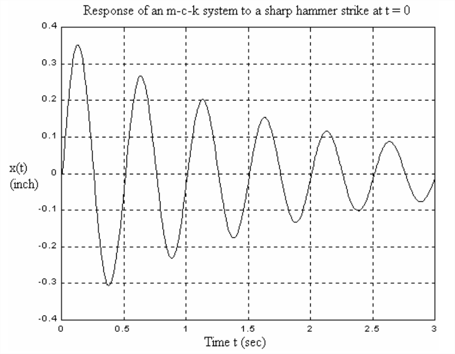
Figure \(\PageIndex{6}\) - For systems with the particular type of right-hand-side dynamics of Equation 9.10.9, we can define a physical constant \(T\) having dimensions of time, then write a modified form of standard ODE Equation 9.2.2 as \(\ddot{x}+2 \zeta \omega_{n} \dot{x}+\omega_{n}^{2} x=\omega_{n}^{2} T \dot{u}(t)\). [You can easily verify, for example, that \(T=\tau_{H}\) for the band-pass filter, Equation 9.10.9.] The pure IC-response of this equation is the same as Equations 9.4.1 and 9.4.2, so let us focus on the forced response and set all ICs = 0. Also, let us assume initially that \(|\zeta|<1\), so that \(\omega_{d}^{2}=\omega_{n}^{2}\left(1-\zeta^{2}\right)>0\)) .
- For this modified ODE, follow the steps from Equations 9.3.2 to 9.3.5, and assume also that \(u(0)=0\). to find \(L[x(t)]=\frac{\omega_{n}^{2} T}{\omega_{d}} \frac{s \omega_{d}}{\left(s+\zeta \omega_{n}\right)^{2}+\omega_{d}^{2}} L[u(t)]\). Next, use a Laplace transform pair developed, in effect, between Equations 9.3.5 and 9.3.9 to solve for \(x(t)\) if the input is step function \(u(t)=U H(t)\). Which of the zero ICs is or is not preserved in this solution?
- Use the inverse transform for step response of part 9.15.1, and the general transform \(L[\dot{f}(t)]=s F(s)-f(0)\) to derive the following inverse transform:\[L^{-1}\left[\frac{s \omega_{d}}{\left(s+\zeta \omega_{n}\right)^{2}+\omega_{d}^{2}}\right]=e^{-\zeta \omega_{n} t}\left(\omega_{d} \cos \omega_{d} t-\zeta \omega_{n} \sin \omega_{d} t\right) \nonumber \]
- Use the result of part 9.15.2 and the inverse convolution transform to write \(\left.x(t)\right|_{I C s=0}\) equations, which involve convolution integrals, that apply for arbitrary input function \(u(t)\).
- Use the result of part 9.15.2 and Equation 8.6.6 to show that the algebraic equation for the unit-impulse-response function (IRF) valid for the modified 2nd order ODE with righthand side dynamics is \(h(t)=\omega_{n}^{2} T e^{-\zeta \omega_{n} t}\left[\cos \omega_{d} t-\left(\zeta \omega_{n} / \omega_{d}\right) \sin \omega_{d} t\right]\). Now use this IRF to write a Duhamel integral equation, Equation 8.7.2, for \(\left.x(t)\right|_{I C s=0}\) that applies for arbitrary input function \(u(t)\).
- The results of parts 9.15.1-9.15.4 apply for an underdamped 2nd order system, \(|\zeta|<1\). But Example 9.10.1 in Section 9.10 shows that an RC band-pass filter, for one, is an overdamped 2nd order system, so we need to convert the previous results to obtain results valid for \(|\zeta|>1\). Use the methods of Section 9.10 to write an algebraic equation for IRF \(h(t)\) and an integral equation for \(\left.x(t)\right|_{I C s=0}\), both valid for the modified overdamped 2nd order ODE with right-hand side dynamics and the latter valid for arbitrary input function \(u(t)\).
- Figure 9.7 includes a curve that is step response of a standard overdamped 2nd order system. Use the methods of Section 9.10 to derive the algebraic equation from which that particular curve was calculated. Answer: \[x(t)=U\left[1-e^{-\zeta \omega_{n} t}\left(\cosh \mu_{d} t+\frac{\zeta \omega_{n}}{\mu_{d}} \sinh \mu_{d} t\right)\right], \text { for } 0 \leq t \text { and } \zeta>1, \mu_{d} \equiv \omega_{n} \sqrt{\zeta^{2}-1} \nonumber \]
- The circuit drawn at right2 consists of three stages, each built around an op-amp, and there is feedback of voltage \(e_{f}(t)\) from the last (right-hand) stage to the first (left-hand) stage, where the input voltage \(e_{i}(t)\) is applied. The circuit output voltage, \(e_{o}(t)\), is the output of the middle stage. The first stage is a summing, inverting integrator; use the methods of Chapter 5 to derive the first ODE, \(e_{m} / R_{c}+e_{f} / R_{b}+e_{i} / R_{a}=-C \dot{e}_{m}\). Next, for the middle stage, an inverting integrator, derive the second ODE, \(e_{m} / R_{b}=-C \dot{e}_{o}\) (homework Problem 5.6); now use the second ODE to substitute for \(e_{m}\) in the first ODE, and differentiate the second ODE and use the result to substitute for \(\dot{e}_{m}\) in the first ODE. The last stage of the circuit is a simple sign inverter, for which \(e_{f}=-e_{o}\) from Equation 5.3.5; substitute for \(e_{f}\) and show that the ODE relating output voltage \(e_{o}(t)\) to input voltage \(e_{i}(t)\) for the entire circuit is \(\ddot{e}_{o}+\frac{1}{R_{c} C} \dot{e}_{o}+\left(\frac{1}{R_{b} C}\right)^{2} e_{o}=\left(\frac{1}{R_{b} C}\right)^{2} \frac{R_{b}}{R_{a}} e_{i}\). Convert this ODE into the standard damped 2nd order form Equation 9.2.2, \(\ddot{e}_{o}+2 \zeta \omega_{n} \dot{e}_{o}+\omega_{n}^{2} e_{o}=\omega_{n}^{2} u(t)\); write specific equations (in terms of this circuit’s resistances, capacitances, and input voltage) for undamped natural frequency \(\omega_{n}\), viscous damping ratio \(\zeta\), and input quantity \(u(t)\).
- One rate gyroscope (Example 9.2 in Section 9.2) has the following rotor parameters: polar rotational inertia \(J_{r}=2.9 \times 10^{-4} \mathrm{kg}-\mathrm{m}^{2}\), and spin rate \(\Omega_{r}=2,100\) revolutions per minute (rpm); also, it has the following gimbal-shaft parameters: polar rotational inertia \(J_{\theta}=2.2 \times 10^{-4} \mathrm{kg}-\mathrm{m}^{2}\), \(J_{\theta}=2.2 \times 10^{-4} \mathrm{kg}-\mathrm{m}^{2}\), and damping constant \(c_{\theta}=0.0046 \mathrm{N}-\mathrm{m} /(\mathrm{rad} / \mathrm{s})\), and stiffness constant \(k_{\theta}=0.096 \mathrm{N}-\mathrm{m} / \mathrm{rad}\). Consider output gimbal-shaft rotation \(\theta(t)\) in response to an input turntable rotational rate that approximates step function \(p(t) \approx P \times H(t)\). (Only a physically impossible ideal impulse moment acting on the turntable could produce an exact step change in rotational rate; therefore, imagine for this problem that a very short but very large moment pulse produces the approximate step function, but use the equations that apply for an exact step function.) For the step magnitude \(P=15\) degrees/s, calculate the following response quantities: pseudo-static gimbal-shaft rotation, \(\theta_{p s}\) (in degrees); and rise time, \(t_{r}\); and peak time, \(t_p\); and maximum overshoot ratio, \(\bar{x}_{p}\). (Partial answer: \(t_{p}=0.174\) s) The theory developed in Example 9.2.2 is accurate only if gimbalshaft rotation \(\theta (t)\) is sufficiently small that \(\cos \theta(t) \approx 1\), say, \(\cos \theta(t)>0.95\). For the parameters in this problem, is this criterion for accuracy satisfied?
- Another type of single-axis gyroscopic sensor is similar to the rate gyro described in Example 9.2.2 of Section 9.2 except that there is no spring to restrain the rotation of the gimbal-shaft assembly, so \(k_{\theta}=0\) in the equations derived in Example 9.2.2. Therefore, the equation of motion becomes effectively a 1st order ODE in dependent variable \(\dot{\theta}(t)\), the rate of gimbal-shaft rotation:\[J_{\theta} \ddot{\theta}+c_{\theta} \dot{\theta}=J_{r} \Omega_{r} p(t) \nonumber \]Observe from the ODE that the pseudo-static response is \((\dot{\theta})_{p s}=\left(J_{r} \Omega_{r} / c_{\theta}\right) p(t)\). But the electrical transducer of this device detects \(\theta(t)\), not \(\dot{\theta}(t)\), which means that the sensed quantity has the form \(\theta(t)=\int_{t} \dot{\theta}(\tau) d \tau=\left(J_{r} \Omega_{r} / c_{\theta}\right) \int_{t} p(\tau) d \tau\). Therefore, this type of sensor is called a rate-integrating gyroscope; its output is proportional, not to the rotational rate, but to the actual rotational angle of the turntable, \(\psi(t)=\int_{t} p(\tau) d \tau\), where \(p \equiv \dot{\psi}\). Consider output gimbal-shaft rotational rate \(\dot{\theta}(t)\) and rotation \(\theta(t)\) in response to an input turntable rotational rate that approximates the following flat pulse of duration \(t_{d}\):\[p(t)=\left\{\begin{array}{l}
0, \quad t<0 \\
P, 0<t<t_{d} \quad, \text { in which magnitude } P \text { is constant } \\
0, \quad t_{d}<t
\end{array}\right. \nonumber \](Only physically impossible ideal impulse moments acting on the turntable could produce exact step changes in rotational rate; therefore, imagine for this problem that very short but very large moment pulses produce the approximate step changes, but use the equations that apply for the exact flat pulse.)- The mathematical solution for response of a standard stable 1st order system to a flat-pulse input is given in homework Problem 6.2.1. Adapt this solution to write response equations for the rate-integrating gyro’s gimbal-shaft rotational rate, \(\dot{\theta}(t)\), given the IC \(\dot{\theta}(0)=0\). Next, integrate appropriately (show all details!) the \(\dot{\theta}(t)\) equations, given the IC \(\theta(0)=0\), to derive the following equations for gimbal-shaft rotation:\[\theta(t)=\left\{\begin{aligned}
b P \tau_{1}\left[t-\tau_{1}\left(1-e^{-t / \tau_{1}}\right)\right], & 0 \leq t \leq t_{d} \\
\theta\left(t_{d}\right)+b P \tau_{1}^{2}\left(1-e^{-t_{d} / \tau_{1}}\right)\left(1-e^{-\left(t-t_{d}\right) / \tau_{1}}\right), & t_{d} \leq t
\end{aligned}\right. \nonumber \]where \(b=J_{r} \Omega_{r} / J_{\theta}\) and \(\tau_{1}=J_{\theta} / c_{\theta}\). - One rate-integrating gyro has the following rotor parameters: polar rotational inertia \(J_{r}=2.9 \times 10^{-4} \mathrm{kg}-\mathrm{m}^{2}\), and spin rate \(\Omega_{r}=420\) revolutions per minute (rpm); also, it has the following gimbal-shaft parameters: polar rotational inertia \(J_{\theta}=8.5 \times 10^{-4} \mathrm{kg}-\mathrm{m}^{2}\), and damping constant \(c_{\theta}=9.2 \times 10^{-3}\) N-m/(rad/s). For the flat-pulse rotational-rate magnitude \(P=5\) degrees/s and pulse duration \(t_{d}=2.5\) s, calculate and plot from the equations of part 9.19.1 the gimbal-shaft rotation \(\theta(t)\) (in degrees) over the time interval \(0 \leq t \leq 5\). The theory developed in Example 9-2 is accurate only if gimbal-shaft rotation \(\theta(t)\) is sufficiently small that \(\cos \theta(t) \approx 1\), say, \(\cos \theta(t)>0.95\). For the parameters in this problem, is this criterion for accuracy satisfied?
- Since \((\dot{\theta})_{p s}=\left(J_{r} \Omega_{r} / c_{\theta}\right) p(t)=\left(J_{r} \Omega_{r} / c_{\theta}\right) \dot{\psi}(t)\), it is clear the rate-integrating gyro’s output is designed to be proportional, as closely as its dynamics permit, to the actual rotational angle of the turntable, i.e., \(\theta(t) \approx\left(J_{r} \Omega_{r} / c_{\theta}\right) \psi(t)\); therefore, the equation that estimates \(\psi(t)\) from the measured gimbal-shaft rotation is \(\psi(t) \approx\left[c_{\theta} /\left(J_{r} \Omega_{r}\right)\right] \theta(t)\). Use your calculated \(\theta(t)\) from part 9.19.2 to calculate and plot the quantity \(\left[c_{\theta} /\left(J_{r} \Omega_{r}\right)\right] \theta(t)\) over the same time interval, \(0 \leq t \leq 5\) s. Next, calculate the actual turntable rotational angle from \(\psi(t)=\int_{0}^{t} p(\tau) d \tau\), given the IC \(\psi(0)=0\), and plot it on the same graph for comparison with \(\left[c_{\theta} /\left(J_{r} \Omega_{r}\right)\right] \theta(t)\). In this case, how well does the rate-integrating gyro follow the actual turntable rotation?
- The mathematical solution for response of a standard stable 1st order system to a flat-pulse input is given in homework Problem 6.2.1. Adapt this solution to write response equations for the rate-integrating gyro’s gimbal-shaft rotational rate, \(\dot{\theta}(t)\), given the IC \(\dot{\theta}(0)=0\). Next, integrate appropriately (show all details!) the \(\dot{\theta}(t)\) equations, given the IC \(\theta(0)=0\), to derive the following equations for gimbal-shaft rotation:\[\theta(t)=\left\{\begin{aligned}
1Base excitation is displacement input imposed at the “ground” or “base” side of the spring instead of directly upon the mass. It is very common to consider base excitation in analyses of earthquake-induced response of buildings, automobile tires rolling over bumpy roads, and vibration isolation of sensitive devices such as delicate payloads in rocket boosters.
2This circuit is essentially the electronic analog computer (see the footnote to homework Problem 5.6) for solving ODE Equation 9.2.2.