10.2: Sampling Theorem

Introduction

With the introduction of the concept of signal sampling, which produces a discrete time signal by selecting the values of the continuous time signal at evenly spaced points in time, it is now possible to discuss one of the most important results in signal processing, the Nyquist-Shannon sampling theorem. Often simply called the sampling theorem, this theorem concerns signals, known as bandlimited signals, with spectra that are zero for all frequencies with absolute value greater than or equal to a certain level. The theorem implies that there is a sufficiently high sampling rate at which a bandlimited signal can be recovered exactly from its samples, which is an important step in the processing of continuous time signals using the tools of discrete time signal processing.

Nyquist-Shannon Sampling Theorem

Statement of the Sampling Theorem

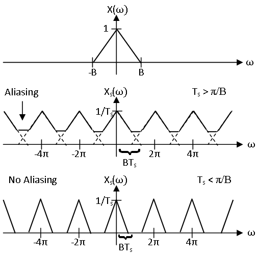
The Nyquist-Shannon sampling theorem concerns signals with continuous time Fourier transforms that are only nonzero on the interval \((−B,B)\) for some constant \(B\). Such a function is said to be bandlimited to \((−B,B)\). Essentially, the sampling theorem has already been implicitly introduced in the previous module concerning sampling. Given a continuous time signals \(x\) with continuous time Fourier transform \(X\), recall that the spectrum \(X_s\) of sampled signal \(x_s\) with sampling period \(T_s\) is given by

\[X_{s}(\omega)=\frac{1}{T_{s}} \sum_{k=-\infty}^{\infty} X\left(\frac{\omega-2 \pi k}{T_{s}}\right). \nonumber \]

It had previously been noted that if \(x\) is bandlimited to \((−\pi/T_s,\pi/T_s)\), the period of \(X_s\) centered about the origin has the same form as \(X\) scaled in frequency since no aliasing occurs. This is illustrated in Figure \(\PageIndex{1}\). Hence, if any two \((−\pi/T_s,\pi/T_s)\) bandlimited continuous time signals sampled to the same signal, they would have the same continuous time Fourier transform and thus be identical. Thus, for each discrete time signal there is a unique \((−\pi/T_s,\pi/T_s)\) bandlimited continuous time signal that samples to the discrete time signal with sampling period \(T_s\). Therefore, this \((−\pi/T_s,\pi/T_s)\) bandlimited signal can be found from the samples by inverting this bijection.

This is the essence of the sampling theorem. More formally, the sampling theorem states the following. If a signal \(x\) is bandlimited to \((−B,B)\), it is completely determined by its samples with sampling rate \(\omega_s=2B\). That is to say, \(x\) can be reconstructed exactly from its samples \(x_s\) with sampling rate \(\omega_s=2B\). The angular frequency \(2B\) is often called the angular Nyquist rate. Equivalently, this can be stated in terms of the sampling period \(T_s=2 \pi / \omega_s\). If a signal \(x\) is bandlimited to \((−B,B)\), it is completely determined by its samples with sampling period \(T_s=\pi/B\). That is to say, \(x\) can be reconstructed exactly from its samples \(x_s\) with sampling period \(T_s\).

Figure \(\PageIndex{1}\): The spectrum of a bandlimited signals is shown as well as the spectra of its samples at rates above and below the Nyquist frequency. As is shown, no aliasing occurs above the Nyquist frequency, and the period of the samples spectrum centered about the origin has the same form as the spectrum of the original signal scaled in frequency. Below the Nyquist frequency, aliasing can occur and causes the spectrum to take a different than the original spectrum.

Proof of the Sampling Theorem

The above discussion has already shown the sampling theorem in an informal and intuitive way that could easily be refined into a formal proof. However, the original proof of the sampling theorem, which will be given here, provides the interesting observation that the samples of a signal with period \(T_s\) provide Fourier series coefficients for the original signal spectrum on \(\left(-\pi / T_{s}, \pi / T_{s}\right)\).

Let \(x\) be a \(\left(-\pi / T_{s}, \pi / T_{s}\right)\) bandlimited signal and \(x_s\) be its samples with sampling period \(T_s\). We can represent \(x\) in terms of its spectrum \(X\) using the inverse continuous time Fourier transform and the fact that \(x\) is bandlimited. The result is

\[x(t)=\frac{1}{2 \pi} \int_{-\pi / T_{x}}^{\pi / T_{s}} X(\omega) e^{j \omega t} d \omega \nonumber \]

This representation of \(x\) may then be sampled with sampling period \(T_s\) to produce

\[x_{s}(n)=x_{s}\left(n T_{s}\right)=\frac{1}{2 \pi} \int_{-\pi / T_{s}}^{\pi / T_{s}} X(\omega) e^{j \omega n T_{s}} d \omega \nonumber \]

Noticing that this indicates that \(x_s(n)\) is the \(n\)th continuous time Fourier series coefficient for \(X(\omega)\) on the interval \(\left(-\pi / T_{s}, \pi / T_{s}\right)\), it is shown that the samples determine the original spectrum \(X(\omega)\) and, by extension, the original signal itself.

Perfect Reconstruction

Another way to show the sampling theorem is to derive the reconstruction formula that gives the original signal \(\tilde{x}=x\) from its samples \(x_s\) with sampling period \(T_s\), provided \(x\) is bandlimited to \(\left(-\pi / T_{s}, \pi / T_{s}\right)\). This is done in the module on perfect reconstruction. However, the result, known as the Whittaker-Shannon reconstruction formula, will be stated here. If the requisite conditions hold, then the perfect reconstruction is given by

\[x(t)=\sum_{n=-\infty}^{\infty} x_{s}(n) \operatorname{sinc}\left(t / T_{s}-n\right) \nonumber \]

where the sinc function is defined as

\[\operatorname{sinc}(t)=\frac{\sin (\pi t)}{\pi t}. \nonumber \]

From this, it is clear that the set

\[\left\{\operatorname{sinc}\left(t / T_{s}-n\right) \: | \: n \in \mathbb{Z}\right\} \nonumber \]

forms an orthogonal basis for the set of \(\left(-\pi / T_{s}, \pi / T_{s}\right)\) bandlimited signals, where the coefficients of a \(\left(-\pi / T_{s}, \pi / T_{s}\right)\) signal in this basis are its samples with sampling period \(T_s\).

Practical Implications

Discrete Time Processing of Continuous Time Signals

The Nyquist-Shannon Sampling Theorem and the Whittaker-Shannon Reconstruction formula enable discrete time processing of continuous time signals. Because any linear time invariant filter performs a multiplication in the frequency domain, the result of applying a linear time invariant filter to a bandlimited signal is an output signal with the same bandlimit. Since sampling a bandlimited continuous time signal above the Nyquist rate produces a discrete time signal with a spectrum of the same form as the original spectrum, a discrete time filter could modify the samples spectrum and perfectly reconstruct the output to produce the same result as a continuous time filter. This allows the use of digital computing power and flexibility to be leveraged in continuous time signal processing as well. This is more thoroughly described in the final module of this chapter.

Psychoacoustics

The properties of human physiology and psychology often inform design choices in technologies meant for interaction with people. For instance, digital devices dealing with sound use sampling rates related to the frequency range of human vocalizations and the frequency range of human auditory sensitivity. Because most of the sounds in human speech concentrate most of their signal energy between 5 Hz and 4 kHz, most telephone systems discard frequencies above 4 kHz and sample at a rate of 8 kHz. Discarding the frequencies greater than or equal to 4 kHz through use of an anti-aliasing filter is important to avoid aliasing, which would negatively impact the quality of the output sound as is described in a later module. Similarly, human hearing is sensitive to frequencies between 20 Hz and 20 kHz. Therefore, sampling rates for general audio waveforms placed on CDs were chosen to be greater than 40 kHz, and all frequency content greater than or equal to some level is discarded. The particular value that was chosen, 44.1 kHz, was selected for other reasons, but the sampling theorem and the range of human hearing provided a lower bound for the range of choices.

Sampling Theorem Summary

The Nyquist-Shannon Sampling Theorem states that a signal bandlimited to \(\left(-\pi / T_{s}, \pi / T_{s}\right)\) can be reconstructed exactly from its samples with sampling period \(T_s\). The Whittaker-Shannon interpolation formula, which will be further described in the section on perfect reconstruction, provides the reconstruction of the unique \(\left(-\pi / T_{s}, \pi / T_{s}\right)\) bandlimited continuous time signal that samples to a given discrete time signal with sampling period \(T_s\). This enables discrete time processing of continuous time signals, which has many powerful applications.