10.7: Discrete Time Processing of Continuous Time Signals

Introduction

Digital computers can process discrete time signals using extremely flexible and powerful algorithms. However, most signals of interest are continuous time signals, which is how data almost always appears in nature. Now that the theory supporting methods for generating a discrete time signal from a continuous time signal through sampling and then perfectly reconstructing the original signal from its samples without error has been discussed, it will be shown how this can be applied to implement continuous time, linear time invariant systems using discrete time, linear time invariant systems. This is of key importance to many modern technologies as it allows the power of digital computing to be leveraged for processing of analog signals.

Discrete Time Processing of Continuous Time Signals

Process Structure

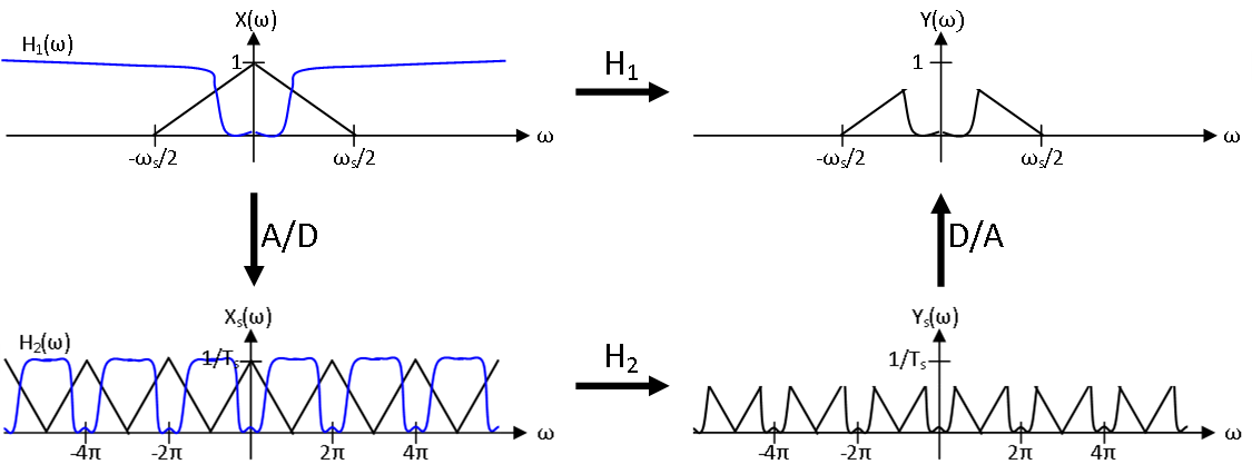
With the aim of processing continuous time signals using a discrete time system, we will now examine one of the most common structures of digital signal processing technologies. As an overview of the approach taken, the original continuous time signal \(x\) is sampled to a discrete time signal \(x_s\) in such a way that the periods of the samples spectrum \(X_s\) is as close as possible in shape to the spectrum of \(X\). Then a discrete time, linear time invariant filter \(H_2\) is applied, which modifies the shape of the samples spectrum \(X_s\) but cannot increase the bandlimit of \(X_s\), to produce another signal \(y_s\). This is reconstructed with a suitable reconstruction filter to produce a continuous time output signal \(y\), thus effectively implementing some continuous time system \(H_1\). This process is illustrated in Figure \(\PageIndex{1}\), and the spectra are shown for a specific case in Figure \(\PageIndex{2}\).

Figure \(\PageIndex{1}\): A block diagram for processing of continuous time signals using discrete time systems is shown.

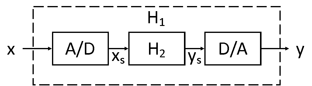
Further discussion about each of these steps is necessary, and we will begin by discussing the analog to digital converter, often denoted by ADC or A/D. It is clear that in order to process a continuous time signal using discrete time techniques, we must sample the signal as an initial step. This is essentially the purpose of the ADC, although there are practical issues that which will be discussed later. An ADC takes a continuous time analog signal as input and produces a discrete time digital signal as output, with the ideal infinite precision case corresponding to sampling. As stated by the Nyquist-Shannon Sampling theorem, in order to retain all information about the original signal, we usually wish sample above the Nyquist frequency \(\omega_s≥2B\) where the original signal is bandlimited to \((−B,B)\). When it is not possible to guarantee this condition, an anti-aliasing filter should be used.

The discrete time filter is where the intentional modifications to the signal information occur. This is commonly done in digital computer software after the signal has been sampled by a hardware ADC and before it is used by a hardware DAC to construct the output. This allows the above setup to be quite flexible in the filter that it implements. If sampling above the Nyquist frequency the. Any modifications that the discrete filter makes to this shape can be passed on to a continuous time signal assuming perfect reconstruction. Consequently, the process described will implement a continuous time, linear time invariant filter. This will be explained in more mathematical detail in the subsequent section. As usual, there are, of course, practical limitations that will be discussed later.

Finally, we will discuss the digital to analog converter, often denoted by DAC or D/A. Since continuous time filters have continuous time inputs and continuous time outputs, we must construct a continuous time signal from our filtered discrete time signal. Assuming that we have sampled a bandlimited at a sufficiently high rate, in the ideal case this would be done using perfect reconstruction through the Whittaker-Shannon interpolation formula. However, there are, once again, practical issues that prevent this from happening that will be discussed later.

Figure \(\PageIndex{2}\): Spectra are shown in black for each step in implementing a continuous time filter using a discrete time filter for a specific signal. The filter frequency responses are shown in blue, and both are meant to have maximum value 1 in spite of the vertical scale that is meant only for the signal spectra. Ideal ADCs and DACs are assumed.

Discrete Time Filter

With some initial discussion of the process illustrated in Figure \(\PageIndex{1}\) complete, the relationship between the continuous time, linear time invariant filter \(H_1\) and the discrete time, linear time invariant filter \(H_2\) can be explored. We will assume the use of ideal, infinite precision ADCs and DACs that perform sampling and perfect reconstruction, respectively, using a sampling rate \(\omega_s=2 \pi /T_s≥2B\) where the input signal \(x\) is bandlimited to \((−B,B)\). Note that these arguments fail if this condition is not met and aliasing occurs. In that case, pre-application of an anti-aliasing filter is necessary for these arguments to hold.

Recall that we have already calculated the spectrum \(X_s\) of the samples \(x_s\) given an input \(x\) with spectrum \(X\) as

\[X_{s}(\omega)=\frac{1}{T_{s}} \sum_{k=-\infty}^{\infty} X\left(\frac{\omega-2 \pi k}{T_{s}}\right) . \nonumber \]

Likewise, the spectrum \(Y_s\) of the samples \(y_s\) given an output \(y\) with spectrum \(Y\) is

\[Y_{s}(\omega)=\frac{1}{T_{s}} \sum_{k=-\infty}^{\infty} Y\left(\frac{\omega-2 \pi k}{T_{s}}\right) . \nonumber \]

From the knowledge that \(y_s=(H_1x)_s=H_2(x_s)\), it follows that

\[\sum_{k=-\infty}^{\infty} H_{1}\left(\frac{\omega-2 \pi k}{T_{s}}\right) X\left(\frac{\omega-2 \pi k}{T_{s}}\right)=H_{2}(\omega) \sum_{k=-\infty}^{\infty} X\left(\frac{\omega-2 \pi k}{T_{s}}\right). \nonumber \]

Because \(X\) is bandlimited to \((−\pi /T_s, \pi /T_s)\), we may conclude that

\[H_{2}(\omega)=\sum_{k=-\infty}^{\infty} H_{1}\left(\frac{\omega-2 \pi k}{T_{s}}\right)(u(\omega-(2 k-1) \pi)-u(\omega-(2 k+1) \pi)). \nonumber \]

More simply stated, \(H_2\) is \(2 \pi\) periodic and \(H_2(\omega)=H_1( \omega /T_s)\) for \(\omega \in[-\pi, \pi)\).

Given a specific continuous time, linear time invariant filter \(H_1\), the above equation solves the system design problem provided we know how to implement \(H_2\). The filter \(H_2\) must be chosen such that it has a frequency response where each period has the same shape as the frequency response of \(H_1\) on \(\left(-\pi / T_{s}, \pi / T_{s}\right)\). This is illustrated in the frequency responses shown in Figure \(\PageIndex{2}\).

We might also want to consider the system analysis problem in which a specific discrete time, linear time invariant filter \(H_2\) is given, and we wish to describe the filter \(H_1\). There are many such filters, but we can describe their frequency responses on \(\left(-\pi / T_{s}, \pi / T_{s}\right)\) using the above equation. Isolating one period of \(H_2(\omega)\) yields the conclusion that \(H_{1}(\omega)=H_{2}\left(\omega T_{s}\right)\) for \(\omega \in\left(-\pi / T_{s}, \pi / T_{s}\right)\). Because \(x\) was assumed to be bandlimited to \(\left(-\pi / T_{s}, \pi / T_{s}\right)\), the value of the frequency response elsewhere is irrelevant.

Practical Considerations

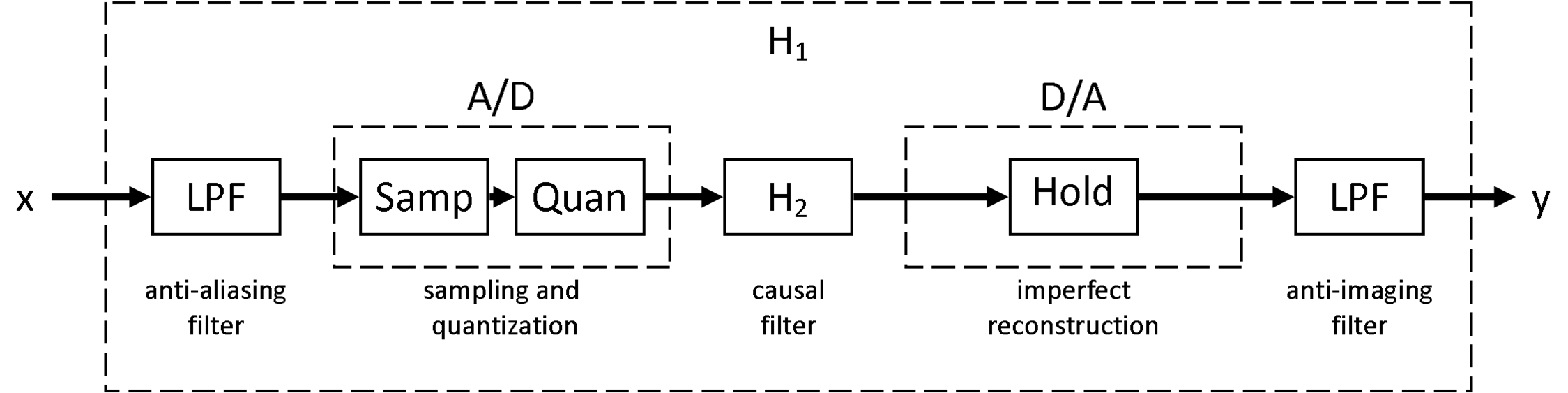
As mentioned before, there are several practical considerations that need to be addressed at each stage of the process shown in Figure \(\PageIndex{1}\). Some of these will be briefly addressed here, and a more complete model of how discrete time processing of continuous time signals appears in Figure \(\PageIndex{3}\).

Figure \(\PageIndex{3}\): A more complete model of how discrete time processing of continuous time signals is implemented in practice. Notice the addition of anti-aliasing and anti-imaging filters to promote input and output bandlimitedness. The ADC is shown to perform sampling with quantization. The digital filter is further specified to be causal. The DAC is shown to perform imperfect reconstruction, a zero order hold in this case.

Anti-Aliasing Filter

In reality, we cannot typically guarantee that the input signal will have a specific bandlimit, and sufficiently high sampling rates cannot necessarily be produced. Since it is imperative that the higher frequency components not be allowed to masquerade as lower frequency components through aliasing, anti-aliasing filters with cutoff frequency less than or equal to \(\omega_s/2\) must be used before the signal is fed into the ADC. The block diagram in Figure \(\PageIndex{3}\) reflects this addition.

As described in the previous section, an ideal lowpass filter removing all energy at frequencies above \(\omega_s/2\) would be optimal. Of course, this is not achievable, so approximations of the ideal lowpass filter with low gain above \(\omega_s/2\) must be accepted. This means that some aliasing is inevitable, but it can be reduced to a mostly insignificant level.

Signal Quantization

In our preceding discussion of discrete time processing of continuous time signals, we had assumed an ideal case in which the ADC performs sampling exactly. However, while an ADC does convert a continuous time signal to a discrete time signal, it also must convert analog values to digital values for use in a digital logic device, a phenomenon called quantization. The ADC subsystem of the block diagram in Figure \(\PageIndex{3}\) reflects this addition.

The data obtained by the ADC must be stored in finitely many bits inside a digital logic device. Thus, there are only finitely many values that a digital sample can take, specifically \(2N\) where \(N\) is the number of bits, while there are uncountably many values an analog sample can take. Hence something must be lost in the quantization process. The result is that quantization limits both the range and precision of the output of the ADC. Both are finite, and improving one at constant number of bits requires sacrificing quality in the other.

Filter Implementability

In real world circumstances, if the input signal is a function of time, the future values of the signal cannot be used to calculate the output. Thus, the digital filter \(H_2\) and the overall system \(H_1\) must be causal. The filter annotation in Figure \(\PageIndex{3}\) reflects this addition. If the desired system is not causal but has impulse response equal to zero before some time \(t_0\), a delay can be introduced to make it causal. However, if this delay is excessive or the impulse response has infinite length, a windowing scheme becomes necessary in order to practically solve the problem. Multiplying by a window to decrease the length of the impulse response can reduce the necessary delay and decrease computational requirements.

Take, for instance the case of the ideal lowpass filter. It is acausal and infinite in length in both directions. Thus, we must satisfy ourselves with an approximation. One might suggest that these approximations could be achieved by truncating the sinc impulse response of the lowpass filter at one of its zeros, effectively windowing it with a rectangular pulse. However, doing so would produce poor results in the frequency domain as the resulting convolution would significantly spread the signal energy. Other windowing functions, of which there are many, spread the signal less in the frequency domain and are thus much more useful for producing these approximations.

Anti-Imaging Filter

In our preceding discussion of discrete time processing of continuous time signals, we had assumed an ideal case in which the DAC performs perfect reconstruction. However, when considering practical matters, it is important to remember that the sinc function, which is used for Whittaker-Shannon interpolation, is infinite in length and acausal. Hence, it would be impossible for an DAC to implement perfect reconstruction.

Instead, the DAC implements a causal zero order hold or other simple reconstruction scheme with respect to the sampling rate \(\omega_s\) used by the ADC. However, doing so will result in a function that is not bandlimited to \((−\omega_s/2,\omega_s/2)\). Therefore, an additional lowpass filter, called an anti-imaging filter, must be applied to the output. The process illustrated in Figure \(\PageIndex{3}\) reflects these additions. The anti-imaging filter attempts to bandlimit the signal to \((−\omega_s/2,\omega_s/2)\), so an ideal lowpass filter would be optimal. However, as has already been stated, this is not possible. Therefore, approximations of the ideal lowpass filter with low gain above \(\omega_s/2\) must be accepted. The anti-imaging filter typically has the same characteristics as the anti-aliasing filter.

Discrete Time Processing of Continuous Time Signals Summary

As has been show, the sampling and reconstruction can be used to implement continuous time systems using discrete time systems, which is very powerful due to the versatility, flexibility, and speed of digital computers. However, there are a large number of practical considerations that must be taken into account when attempting to accomplish this, including quantization noise and anti-aliasing in the analog to digital converter, filter implementability in the discrete time filter, and reconstruction windowing and associated issues in the digital to analog converter. Many modern technologies address these issues and make use of this process.