
13.3: Deriving the Fast Fourier Transform
- Page ID
- 22923

To derive the FFT, we assume that the signal's duration is a power of two: \(N=2^l\). Consider what happens to the even-numbered and odd-numbered elements of the sequence in the DFT calculation.
\[\begin{align}S(k) &=s(0)+s(2) e^{(-j) \frac{2 \pi 2 k}{N}}+\ldots+s(N-2) e^{(-j) \frac{2 \pi(N-2) k}{N}}+s(1) e^{(-j) \frac{2 \pi k}{N}}+s(3) e^{(-j) \frac{2 \pi \times (2+1) k}{N}}+\ldots+s(N-1) e^{(-j) \frac{2 \pi(N-2+1) k}{N}} \nonumber \\ &=s(0)+s(2)e^{(-j)\frac{2\pi k}{\frac{N}{2}}} + \ldots + s(N-2)e^{(-j) \frac{2 \pi\left(\frac{N}{2}-1\right) k}{\frac{N}{2}}} +\left( s(1)+s(3) e^{(-j) \frac{2 \pi k}{\frac{N}{2}}}+\dots+s(N-1) e^{(-j) \frac{2 \pi\left(\frac{N}{2}-1\right) k}{\frac{N}{2}}}\right) e^{\frac{-(j 2 \pi k)}{N}} \end{align} \nonumber \]
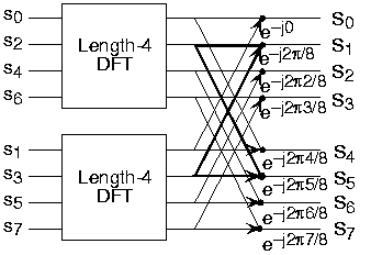
Each term in square brackets has the form of a \(\frac{N}{2}\) -length DFT. The first one is a DFT of the even-numbered elements, and the second of the odd-numbered elements. The first DFT is combined with the second multiplied by the complex exponential \(e^{\frac{-(j2\pi k)}{N}}\). The half-length transforms are each evaluated at frequency indices \(k \in\{0, \ldots, N-1\}\). Normally, the number of frequency indices in a DFT calculation range between zero and the transform length minus one. The computational advantage of the FFT comes from recognizing the periodic nature of the discrete Fourier transform. The FFT simply reuses the computations made in the half-length transforms and combines them through additions and the multiplication by \(e^{\frac{-(j2\pi k)}{N}}\), which is not periodic over \(\frac{N}{2}\), to rewrite the length-N DFT. Figure \(\PageIndex{1}\) illustrates this decomposition. As it stands, we now compute two length- \(\frac{N}{2}\) transforms (complexity \(2O(\frac{N^2}{4})\)), multiply one of them by the complex exponential (complexity \(O(N)\)), and add the results (complexity \(O(N)\)). At this point, the total complexity is still dominated by the half-length DFT calculations, but the proportionality coefficient has been reduced.
Now for the fun. Because \(N=2^l\), each of the half-length transforms can be reduced to two quarter-length transforms, each of these to two eighth-length ones, etc. This decomposition continues until we are left with length-2 transforms. This transform is quite simple, involving only additions. Thus, the first stage of the FFT has \(\frac{N}{2}\) length-2 transforms (see the bottom part of Figure \(\PageIndex{1}\)). Pairs of these transforms are combined by adding one to the other multiplied by a complex exponential. Each pair requires 4 additions and 4 multiplications, giving a total number of computations equaling \(8 \frac{N}{4}=\frac{N}{2}\). This number of computations does not change from stage to stage. Because the number of stages, the number of times the length can be divided by two, equals \(\log_2 N\), the complexity of the FFT is \(O(N \log N)\).
Length-8 DFT decomposition
 (a)
(a)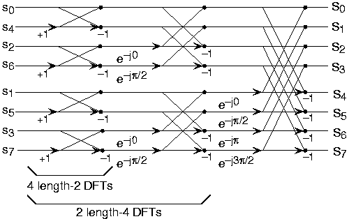 (b)
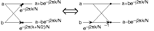
(b)Doing an example will make computational savings more obvious. Let's look at the details of a length-8 DFT. As shown on Figure \(\PageIndex{1}\), we first decompose the DFT into two length-4 DFTs, with the outputs added and subtracted together in pairs. Considering Figure \(\PageIndex{1}\) as the frequency index goes from 0 through 7, we recycle values from the length-4 DFTs into the final calculation because of the periodicity of the DFT output. Examining how pairs of outputs are collected together, we create the basic computational element known as a butterfly (Figure \(\PageIndex{2}\)).
By considering together the computations involving common output frequencies from the two half-length DFTs, we see that the two complex multiplies are related to each other, and we can reduce our computational work even further. By further decomposing the length-4 DFTs into two length-2 DFTs and combining their outputs, we arrive at the diagram summarizing the length-8 fast Fourier transform (Figure \(\PageIndex{1}\)). Although most of the complex multiplies are quite simple (multiplying by \(e^{-(j \pi)}\) means negating real and imaginary parts), let's count those for purposes of evaluating the complexity as full complex multiplies. We have \(\frac{N}{2}=4\) complex multiplies and \(2N=16\) additions for each stage and \(\log_2 N = 3\) stages, making the number of basic computations \(\frac{3N}{2}\log_2 N\) as predicted.
Exercise \(\PageIndex{1}\)
Note that the ordering of the input sequence in the two parts of Figure \(\PageIndex{1}\) aren't quite the same. Why not? How is the ordering determined?
- Answer
-
The upper panel has not used the FFT algorithm to compute the length-4 DFTs while the lower one has. The ordering is determined by the algorithm.
Other "fast" algorithms were discovered, all of which make use of how many common factors the transform length N has. In number theory, the number of prime factors a given integer has measures how composite it is. The numbers \(16\) and \(81\) are highly composite (equaling \(2^4\) and \(3^4\) respectively), the number \(18\) is less so (\(2^1 3^2\) ), and \(17\) not at all (it's prime). In over thirty years of Fourier transform algorithm development, the original Cooley-Tukey algorithm is far and away the most frequently used. It is so computationally efficient that power-of-two transform lengths are frequently used regardless of what the actual length of the data.