
13.4: Matched Filter Detector
- Page ID
- 22924

Introduction
A great many applications in signal processing, image processing, and beyond involve determining the presence and location of a target signal within some other signal. A radar system, for example, searches for copies of a transmitted radar pulse in order to determine the presence of and distance to reflective objects such as buildings or aircraft. A communication system searches for copies of waveforms representing digital 0s and 1s in order to receive a message.
Two key mathematical tools that contribute to these applications are inner products and the Cauchy-Schwarz inequality. As is shown in the module on the Cauchy-Schwarz inequality, the expression \(\left|\left\langle\frac{x}{|| x||}, \frac{y}{\|y\|}\right\rangle\right|\) attains its upper bound, which is 1, when \(y=ax\) for some scalar \(a\) in a real or complex field. The lower bound, which is 0, is attained when \(x\) and \(y\) are orthogonal. In informal intuition, this means that the expression is maximized when the vectors \(x\) and \(y\) have the same shape or pattern and minimized when \(x\) and \(y\) are very different. A pair of vectors with similar but unequal shapes or patterns will produce relatively large value of the expression less than 1, and a pair of vectors with very different but not orthogonal shapes or patterns will produce relatively small values of the expression greater than 0. Thus, the above expression carries with it a notion of the degree to which two signals are “alike”, the magnitude of the normalized correlation between the signals in the case of the standard inner products.
This concept can be extremely useful. For instance consider a situation in which we wish to determine which signal, if any, from a set \(X\) of signals most resembles a particular signal \(y\). In order to accomplish this, we might evaluate the above expression for every signal \(x \in X\), choosing the one that results in maxima provided that those maxima are above some threshold of “likeness”. This is the idea behind the matched filter detector, which compares a set of signals against a target signal using the above expression in order to determine which is most like the target signal.
Matched Filter Detector Theory
Signal Comparison
The simplest variant of the matched filter detector scheme would be to find the member signal in a set \(X\) of signals that most closely matches a target signal \(y\). Thus, for every \(x \in X\) we wish to evaluate
\[m(x, y)=\left|\left\langle\frac{x}{|| x||}, \frac{y}{\|y\|}\right\rangle\right| \nonumber \]
in order to compare every member of \(X\) to the target signal \(y\). Since the member of \(X\) which most closely matches the target signal \(y\) is desired, ultimately we wish to evaluate
\[x_{m}=\operatorname{argmax} _{x \in X}\left|\left\langle\frac{x}{\|x\|}, \frac{y}{\|y\|}\right\rangle\right| \nonumber \]
Note that the target signal does not technically need to be normalized to produce a maximum, but gives the desirable property that \(m(x,y)\) is bounded to \([0,1]\).
The element \(x_{m} \in X\) that produces the maximum value of \(m(x,y)\) is not necessarily unique, so there may be more than one matching signal in \(X\). Additionally, the signal \(x_m \in X\) producing the maximum value of \(m(x,y)\) may not produce a very large value of \(m(x,y)\) and thus not be very much like the target signal \(y\). Hence, another matched filter scheme might identify the argument producing the maximum but only above a certain threshold, returning no matching signals in \(X\) if the maximum is below the threshold. There also may be a signal \(x \in X\) that produces a large value of \(m(x,y)\) and thus has a high degree of “likeness” to \(y\) but does not produce the maximum value of \(m(x,y)\). Thus, yet another matched filter scheme might identify all signals in \(X\) producing local maxima that are above a certain threshold.
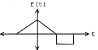
Example \(\PageIndex{1}\)
For example, consider the target signal given in Figure \(\PageIndex{1}\) and the set of two signals given in Figure \(\PageIndex{2}\). By inspection, it is clear that the signal \(g_2\) is most like the target signal \(f\). However, to make that conclusion mathematically, we use the matched filter detector with the \(L_2\) inner product. If we were to actually make the necessary computations, we would first normalize each signal and then compute the necessary inner products in order to compare the signals in \(X\) with the target signal \(f\). We would notice that the absolute value of the inner product for \(g_2\) with \(f\) when normalized is greater than the absolute value of the inner product of \(g_1\) with \(f\) when normalized, mathematically stated as
\[g_{2}=\operatorname{arg max}_{x \in\left\{g_{1}, g_{2}\right\}}\left|\left\langle\frac{x}{\| x||}, \frac{f}{\|f\|}\right\rangle\right| \nonumber \]
Candidate Signals
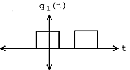 (a)
(a)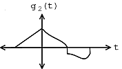 (b)
(b)Pattern Detection
A somewhat more involved matched filter detector scheme would involve attempting to match a target time limited signal \(y=f\) to a set of of time shifted and windowed versions of a single signal \(X=\left\{w S_{t} g \mid t \in \mathbb{R}\right\}\) indexed by \(\mathbb{R}\). The windowing funtion is given by \(w(t)=u\left(t-t_{1}\right)-u\left(t-t_{2}\right)\) where \(\left[t_{1}, t_{2}\right]\) is the interval to which \(f\) is time limited. This scheme could be used to find portions of \(g\) that have the same shape as \(f\). If the absolute value of the inner product of the normalized versions of \(f\) and \(w S_{t} g\) is large, which is the absolute value of the normalized correlation for standard inner products, then \(g\) has a high degree of “likeness” to \(f\) on the interval to which \(f\) is time limited but left shifted by \(t\). Of course, if \(f\) is not time limited, it means that the entire signal has a high degree of “likeness” to \(f\) left shifted by \(t\).
Thus, in order to determine the most likely locations of a signal with the same shape as the target signal \(f\) in a signal \(g\) we wish to compute
\[t_{m}=\operatorname{argmax}_{t \in \mathbb{R}} \mid\left\langle\frac{f}{\|f\|}, \frac{w S_{t} g}{\left\|w S_{t} g\right\|}\right\rangle \nonumber \]
to provide the desired shift. Assuming the inner product space examined is \(L_2\) (\(\mathbb{R}\) (similar results hold for \(L_{2}(\mathbb{R}[a, b))\), \(l_2(\mathbb{Z})\), and \(l_{2}(\mathbb{Z}[a, b))\)), this produces
\[t_{m}=\operatorname{argmax}_{t \in \mathbb{R}}\left|\frac{1}{\|f\|\left\|w S_{t} g\right\|} \int_{-\infty}^{\infty} f(\tau) w(\tau) \overline{g(\tau-t)} d \tau\right| \nonumber \]
Since \(f\) and \(w\) are time limited to the same interval
\[t_{m}=\operatorname{argmax}_{t \in \mathbb{R}}\left|\frac{1}{\|f\|\left\|w S_{t} g\right\|} \int_{t_{1}}^{t_{2}} f(\tau) \overline{g(\tau-t)} d \tau\right| \nonumber \]
Making the substitution \(h(t)=\overline{g(-t)}\),
\[t_{m}=\operatorname{argmax}_{t \in \mathbb{R}}\left|\frac{1}{\|f\|\left\|w S_{t} g\right\|} \int_{t_{1}}^{t_{2}} f(\tau) h(t-\tau) d \tau\right|. \nonumber \]
Noting that this expression contains a convolution operation
\[t_{m}=\operatorname{argmax}_{t \in \mathbb{R}}\left|\frac{(f * h)(t)}{\|f\|\left\|w S_{t} g\right\|}\right| \nonumber \]
where \(h\) is the conjugate of the time reversed version of \(g\) defined by \(h(t)=\overline{g(-t)}\).
In the special case in which the target signal \(f\) is not time limited, \(w\) has unit value on the entire real line. Thus, the norm can be evaluated as \(\left\|w S_{t} g\right\|=\left\|S_{t} g\right\|=\|g\|=\|h\|\). Therefore, the function reduces to \(t_{m}=\operatorname{argmax}_{t \in \mathbb{R}} \frac{\left(f * h\right)(t)}{\|f\|\left\|h\right\|}\) where \(h(t)=\overline{g(-t)}\). The function \(f * g=\frac{\left(f * h\right)(t)}{\|f\|\left\| h\right\|}\) is known as the normalized cross-correlation of \(f\) and \(g\).
Hence, this matched filter scheme can be implemented as a convolution. Therefore, it may be expedient to implement it in the frequency domain. Similar results hold for the \(L_{2}(\mathbb{R}[a, b))\), \(l_{2}(\mathbb{Z})\), and \(l_{2}(\mathbb{Z}[a, b])\) spaces. It is especially useful to implement the \(l_{2}(\mathbb{Z}[a, b])\) cases in the frequency domain as the power of the Fast Fourier Transform algorithm can be leveraged to quickly perform the computations in a computer program. In the \(L_{2}(\mathbb{R}[a, b))\) and \(l_{2}(\mathbb{Z}[a, b])\) cases, care must be taken to zero pad the signal if wrap-around effects are not desired. Similar results also hold for spaces on higher dimensional intervals with the same inner products.
Of course, there is not necessarily exactly one instance of a target signal in a given signal. There could be one instance, more than one instance, or no instance of a target signal. Therefore, it is often more practical to identify all shifts corresponding to local maxima that are above a certain threshold.
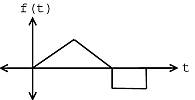
Example \(\PageIndex{2}\)
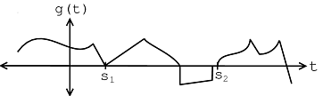
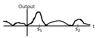
The signal in Figure \(\PageIndex{4}\) contains an instance of the template signal seen in Figure \(\PageIndex{3}\) beginning at time \(t=s_1\) as shown by the plot in Figure \(\PageIndex{5}\). Therefore,
\[s_{1}=\operatorname{argmax}_{t \in \mathbb{R}}\left|\left\langle\frac{f}{\|f\|}, \frac{w S_{t} g}{\left\|w S_{t} g\right\|}\right\rangle\right|. \nonumber \]
Practical Applications
Image Detection
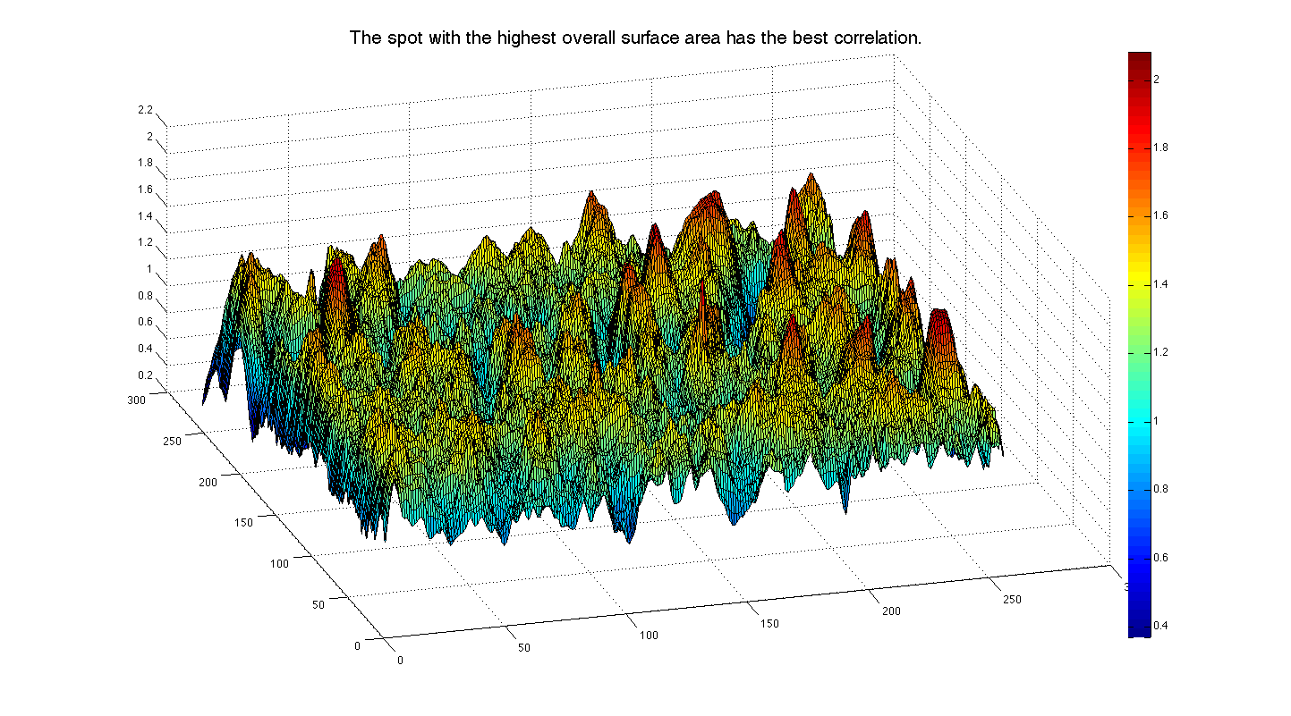
Matched Filtering is used in image processing to detect a template image within a reference image. This has real-word applications in verifying fingerprints for security or in verifying someone's photo. As a simple example, we can turn to the ever-popular "Where's Waldo?" books (known as Wally in the UK!), where the reader is tasked with finding the specific face of Waldo/Wally in a confusing background rife with look-alikes! If we are given the template head and a reference image, we can run a two dimensional convolution of the template image across the reference image to obtain a three dimensional convolution map, Figure \(\PageIndex{6(a)}\), where the height of the convolution map is determined by the degree of correlation, higher being more correlated. Finding our target then becomes a matter of determining the spot where the local surface area is highest. The process is demonstrated in Figure \(\PageIndex{6(b)}\). In the field of image processing, this matched filter-based process is known as template matching.
 (a)
(a)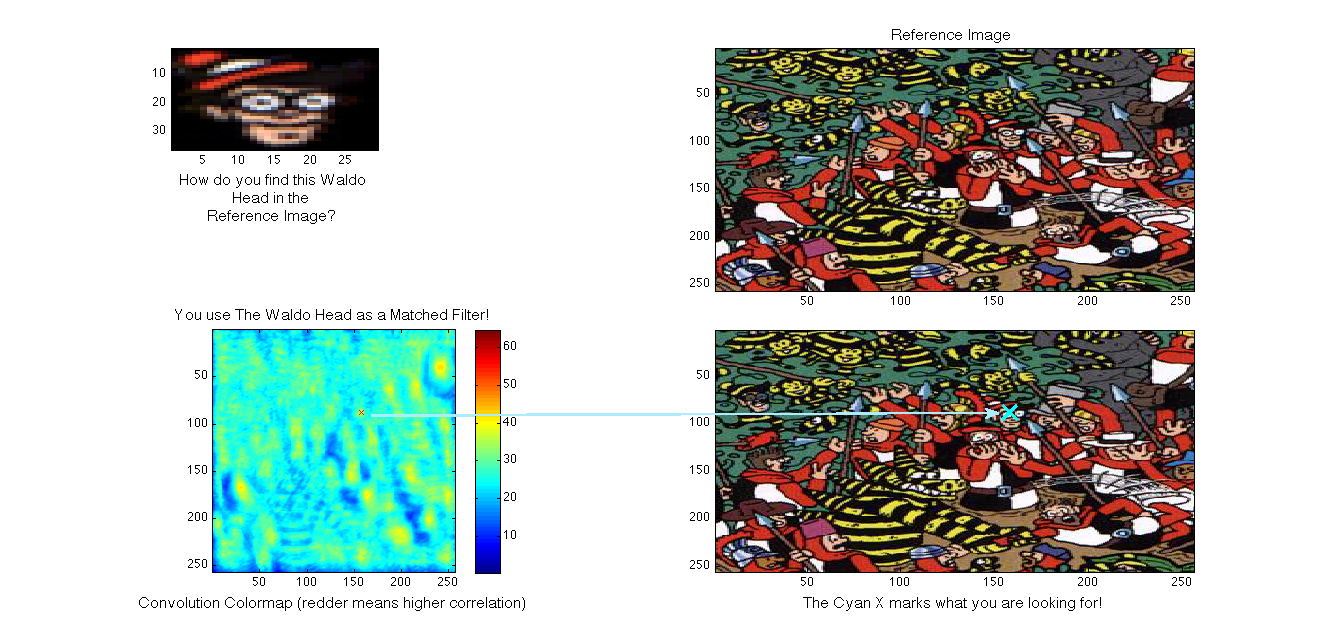 (b)
(b)then we could easily develop a program to find the closest resemblance to the image of Waldo's head in the larger picture. We would simply implement our same match filter algorithm: take the inner products at each shift and see how large our resulting answers are. This idea was implemented on this same picture for a Signals and Systems Project at Rice University (click the link to learn more).
Exercise \(\PageIndex{1}\): Pros and Cons
What are the advantages of the matched filter algorithm to image detection? What are the drawbacks of this method?
- Answer
-
This algorithm is very simple and thus easy to code. However, it is susceptible to certain types of noise - for example, it would be difficult to find Waldo if his face was rotated, flipped, larger or smaller than expected, or distorted in some other way.
Communications Systems
Matched filter detectors are also commonly used in Communications Systems. In fact, they are the optimal detectors in Gaussian noise. Signals in the real-world are often distorted by the environment around them, so there is a constant struggle to develop ways to be able to receive a distorted signal and then be able to filter it in some way to determine what the original signal was. Matched filters provide one way to compare a received signal with two possible original ("template") signals and determine which one is the closest match to the received signal.
For example, below we have a simplified example of Frequency Shift Keying (FSK) where we having the following coding for '1' and '0':
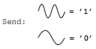
Based on the above coding, we can create digital signals based on 0's and 1's by putting together the above two "codes" in an infinite number of ways. For this example we will transmit a basic 3-bit number, 101, which is displayed in Figure \(\PageIndex{8}\):
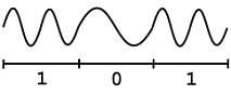
Now, the signal picture above represents our original signal that will be transmitted over some communication system, which will inevitably pass through the "communications channel," the part of the system that will distort and alter our signal. As long as the noise is not too great, our matched filter should keep us from having to worry about these changes to our transmitted signal. Once this signal has been received, we will pass the noisy signal through a simple system, similar to the simplified version shown in Figure \(\PageIndex{9}\):
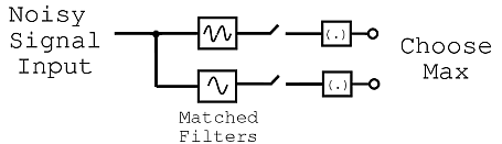
Figure \(\PageIndex{9}\) basically shows that our noisy signal will be passed in (we will assume that it passes in one "bit" at a time) and this signal will be split and passed to two different matched filter detectors. Each one will compare the noisy, received signal to one of the two codes we defined for '1' and '0.' Then this value will be passed on and whichever value is higher (i.e. whichever FSK code signal the noisy signal most resembles) will be the value that the receiver takes. For example, the first bit that will be sent through will be a '1' so the upper level of the block diagram will have a higher value, thus denoting that a '1' was sent by the signal, even though the signal may appear very noisy and distorted.
The interactive example below supposes that our transmitter sends 1000 bits, plotting how many of those bits are received and interpreted correctly as either 1s and 0s, and also keeps a tally of how many are accidentally misinterpreted. You can play around with the distance between the energy of the "1" and the "0" (discriminability), the degree of noise present in the channel, and the location of the criterion (threshold) to get a feel for the basics of signal detection theory.
Example \(\PageIndex{3}\)
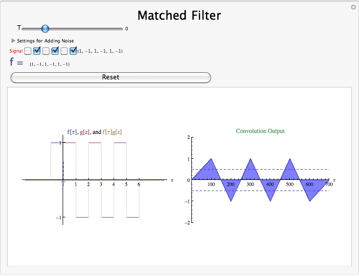
Let's use a matched filter to find the "0" bits in a simple signal.
Let's use the signal \(s_1(t)\) from Example \(\PageIndex{1}\) to represent the bits. \(s_1(t)\) represents 0, while \(-s_1(t)\) represents 1.
\(0 \Rightarrow(b=1) \Rightarrow\left(s_{1}(t)=s(t)\right)\) for \(0≤t≤T\)
\(1 \Rightarrow(b=-1) \Rightarrow\left(s_{2}(t)=-s(t)\right)\) for \(0≤t≤T\)
\[X_{t}=\sum_{i=-P}^{P} b_{i} s(t-i T) \nonumber \]
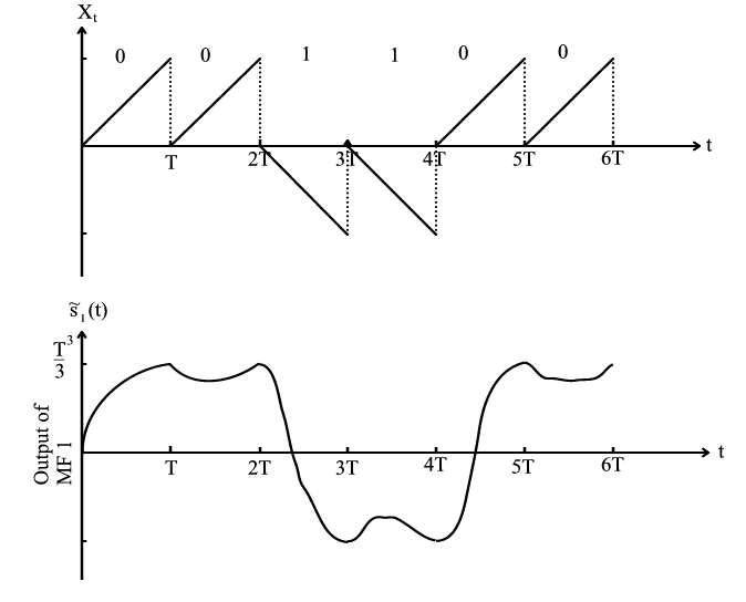
Figure \(\PageIndex{10}\)
The matched filter output clearly shows the location of the "0" bits.
Radar
One of the first, and more intriguing forms of communication that used the matched filter concept was radar. A known electromagnetic signal is sent out by a transmitter at a target and reflected off of the target back to the sender with a time delay proportional to the distance between target and sender. This scaled, time-shifted signal is then convolved with the original template signal, and the time at which the output of this convolution is highest is noted.
This technology proved vital in the 1940s for the powers that possessed it. A short set of videos below shows the basics of how the technology works, its applications, and its impact in World War 2.
Figure \(\PageIndex{11}\)
See the video in Figure \(\PageIndex{12}\) for an analysis of the same basic principle being applied to adaptive cruise control systems for the modern car.
Matched Filter Demonstration
Matched Filter Summary
As can be seen, the matched filter detector is an important signal processing application, rich both in theoretical concepts and in practical applications. The matched filter supports a wide array of uses related to pattern recognition, including image detection, frequency shift keying demodulation, and radar signal interpretation. Despite this diversity of purpose, all matched filter applications operate in essentially the same way. Every member of some set of signals is compared to a target signal by evaluating the absolute value of the inner product of the the two signals after normalization. However, the signal sets and result interpretations are application specific.