2.5: Chapter 2 Homework

1. Refer to Euler’s equation, Equation 2.1.12, which is \(e^{j \theta}=\cos \theta+j \sin \theta\). The cosine is an even (symmetric) function, \(\cos (-\theta)=\cos \theta\), and the sine is an odd (antisymmetric) function, \(\sin (-\theta)=-\sin \theta\), so the conjugate to Euler’s equation is \[e^{-j \theta}=e^{j(-\theta)}=\cos (-\theta)+j \sin (-\theta)=\cos \theta-j \sin \theta \nonumber \]
   1. Add the conjugate to Euler’s equation to prove \(\cos \theta=\frac{e^{j \theta}+e^{-j \theta}}{2}\). Subtract the conjugate from Euler’s equation to prove \(\sin \theta=\frac{e^{j \theta}-e^{-j \theta}}{2 j}\).
   2. Use the results of part 2.1.1 to prove the trigonometric identities \(\cos ^{2} \theta=\frac{1}{2}(1+\cos 2 \theta)\) and \(\sin ^{2} \theta=\frac{1}{2}(1-\cos 2 \theta)\). Use these results to prove \(\cos ^{2} \theta-\sin ^{2} \theta=\cos 2 \theta\).
   3. Use the results of part 2.1.1 to prove the identity \(\sin \theta \times \cos \theta=\frac{1}{2} \sin 2 \theta\).
2. Given the following complex numbers:

   First, express the complex number in rectangular form, \(z=\operatorname{Re}(z)+j \operatorname{Im}(z)\), where \(\operatorname{Re}(z)\) and \(\operatorname{Im}(z)\) are real numbers. Next, express the complex number in polar form \(r e^{j \theta}\), that is, calculate by hand and calculator the radius \(r\) and the phase angle \(\theta\), where \(\theta\) is in degrees, −180° \(\leq\) \(\theta\) < +180°. You may check your hand calculations by using the abs and angle commands appropriately in MATLAB.

   1. \(\frac{1}{-0.4-j 0.3}\)
   2. \(5 j \times(2-j)\)
   3. \(\frac{0.7-j 2.4}{0.5+j 1.2}\)
   4. \(\frac{-10+j 5}{0.6+j 0.8}\)
3. Given: two complex numbers expressed in polar form \(z_{1}=r_{1} e^{j \theta_{1}}\) and \(z_{2}=r_{2} e^{j \theta_{2}}\), with \(r_1\), \(r_2\), \(\theta_1\),and \(\theta_2\) all real numbers.
   1. Use complex arithmetic with complex numbers in polar form to show that the conjugate of a product equals the product of conjugates, which is expressed in equation form as \(\bar{\left(z_{1} \times z_{2}\right)}=\bar{z}_{1} \times \bar{z}_{2}
   2. Use complex arithmetic with complex numbers in polar form to show that the conjugate of a quotient equals the quotient of conjugates, which is expressed in equation form as \(\bar{\left(z_{1} / z_{2}\right)}=\bar{z}_{1} / \bar{z}_{2}\)
4. Express a complex number in rectangular form, \(z=x+j y\), and prove the following identity: \(z+\bar{z}=2 \operatorname{Re}(z)=2 x\).
5. Given: complex numbers \(A=A_{r}+j A_{i}\) and \(B=B_{r}+j B_{i}\) (\(A_r\), \(A_i\), \(B_r\), \(B_i\) all real) and complex variable \(z=x+j y\) (with real, non-zero values of \(x\) and \(y\), which are independent of each other), in the equation \(C=A z+B \bar{z}\).

   Prove: use complex arithmetic with complex values in rectangular form to show that \(C\) can be real, \(C=C_{r}+j 0\), only if \(B=\bar{A}\). (Note that you can also prove this by applying the results of homework Problems 2.3.1 and 2.4.)

6. The following complex function will arise when we study the frequency response of a 2^nd order system: \(Z(\beta)=\frac{1}{\left(1-\beta^{2}\right)+j 2 \zeta \beta}\), in which \(\beta\) is a positive, real, dimensionless forcing frequency (not dimensional frequency \(\omega\)), and \(\zeta\) is a positive, real, dimensionless ratio that represents viscous damping.
   1. Convert the \(\mathrm{Z}(\beta)\) equation above into polar form \(\mathrm{Z}(\beta)=r(\beta) e^{j \theta(\beta)}\). In particular, carry out the detailed algebraic steps to show that the magnitude and phase angle are \(r(\beta)=\frac{1}{\sqrt{\left(1-\beta^{2}\right)^{2}+(2 \zeta \beta)^{2}}}\) and \(\theta(\beta)=\tan ^{-1}\left(\frac{-2 \zeta \beta}{1-\beta^{2}}\right)\).
   2. Calculate values of the magnitude and phase angle for several values of forcing frequency \(\beta\) and for two values of damping ratio \(\zeta\) (specifics below). Make these calculations with a hand calculator, not with MATLAB or some other computer software (although you may check your hand calculations with computer software). These calculations will give you a small preview of frequency response, and (especially) they should help you to understand the care required when you evaluate the four-quadrant arctangent. Specifically, for each of the damping ratios \(\zeta\) = 0 and \(\zeta\) = 0.1 (or another value assigned by your instructor), calculate the quantities in the empty cells of the table below (to at least three significant figures, preferably four, but no more); also, calculate phase angles using the standard engineering convention, −180° \(\leq\) \(\theta\) < +180°, not 0° \(\leq\) \(\theta\) < +360°.

      Hints for the \(\zeta\) = 0 case: (1) for the \(r(\beta)\) calculations, recognize that the equation requires \(r(\beta)\) > 0, even if \(\beta\) > 1; (2) for the \(\theta(\beta)\) calculations, imagine that \(\zeta\) has an extremely small, positive value, say \(\zeta\) = +1 \(\times\) 10^-10.

      

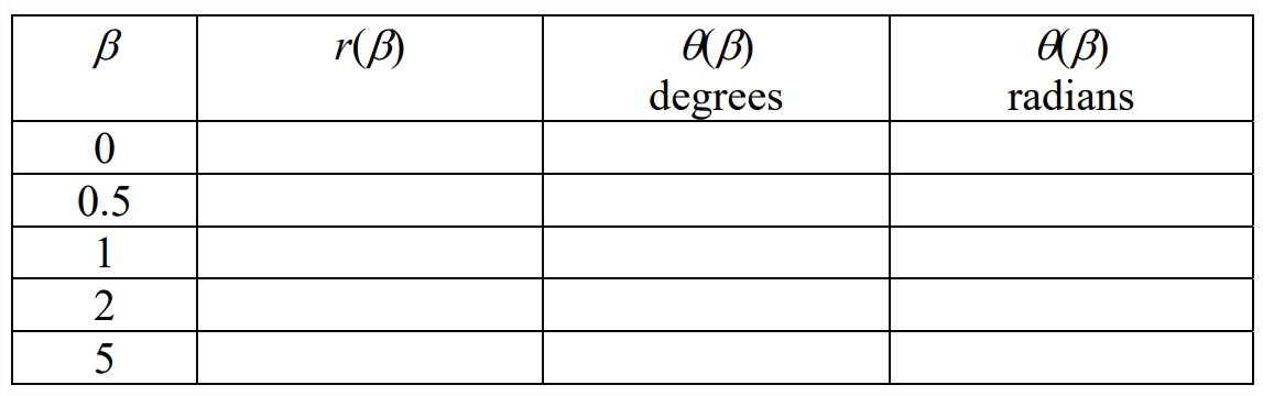
      Figure \(\PageIndex{1}\)

7. Prove Equation 2.2.11, \(L[\ddot{f}(t)]=s^{2} F(s)-s f(0)-\dot{f}(0)\): first define \(g(t)=\dot{f}(t)\); now use the fundamental equation (2-15b) twice, first as \(G(s)=L[\dot{f}]=s F(s)-f(0)\), and then as \(L[\dot{g}]=s G(s)-g(0)\).
8. Consider the Laplace transform shown below, both in the first form, which is derived directly from an ODE, and in a partial-fraction expansion, \[F(s)=\left(\frac{1}{s-a}\right)\left(\frac{1}{s-j \omega}+\frac{1}{s+j \omega}\right)=\frac{C_{1}}{s-a}+\frac{C_{2}}{s-j \omega}+\frac{C_{3}}{s+j \omega} \nonumber \] in which \(a\) and \(\omega\) are real constants. Find residues \(C_1\), \(C_2\), and \(C_3\) in terms of \(a\) and show that \(C_1\) is real. Use the labor-saving method directly, without first completing the products in the form derived from an ODE.
9. Find the inverse Laplace transform \(f(t)\), \(t\) \(\leq\) 0, for the given function \(F(s)\) below. First use partial-fraction expansion to express \(F(s)\) as a sum of simple quotients, and then apply the appropriate inverse transformation equations. Also, find the values of any zeros and poles of \(F(s)\).
   1. \(F(s)=\frac{s+3}{(s+1)(s+5)}\) [Answer: \(f(t)=\frac{1}{2}\left(e^{-t}+e^{-5 t}\right), t \geq 0\)]
   2. \(F(s)=\frac{2(s+1)}{s(s+3)(s+4)}\) [Answer: \(f(t)=\frac{1}{6}+\frac{4}{3} e^{-3 t}-\frac{3}{2} e^{-4 t}, t \geq 0\)]
10. Derive the Laplace transform \(L[\cos \omega t]=\frac{s}{s^{2}+\omega^{2}}\). Follow the same procedure, with appropriate changes in details, as the derivation of \(L[\sin \omega t]\), Equation 2.4.7. Show all steps, just as in the derivation of \(L[\sin \omega t]\).
11. Solution Equation 2.2.26 of ODE problem Equation 2.2.3 was derived by Laplace transformation, a technique that is probably new to you, so you might be a little skeptical. To convince yourself that Equation 2.2.26 is indeed the correct solution of Equation 2.2.3, substitute Equation 2.2.26 back into the ODE and IC of Equation 2.2.3, and show that the original equations are satisfied. This method can always be used to check the correctness of an ODE solution.
12. Consider the standard 1^st order ODE \(\dot{x}-a x=b u(t)\) with IC \(x(0) \equiv x_{0}\). Use Laplace transformation to solve for \(x(t)\) with the \(u(t)\) functions given below. It will ease your algebraic burden greatly if you will make liberal use of the identities involving complex numbers proved in homework Problems 2.3 and 2.4. Also, use where appropriate the transforms of \(\sin \omega t\) from Equation 2.4.7 and \(\cos \omega t\) from Equation 2.4.8 or homework Problem 2.10.
    1. Let \(u(t)=U \sin \omega t\), \(t>0\), where \(U\) is a constant amplitude.

       [Answer: \(x(t)=x_{0} e^{a t}+\frac{b U \omega}{\omega^{2}+a^{2}}\left(e^{a t}-\frac{a}{\omega} \sin \omega t-\cos \omega t\right)\), \(t \geq 0\)]

    2. Let \(u(t)=U \cos \omega t\), \(t > 0\), where \(U\) is a constant amplitude.

       [Answer: \(x(t)=x_{0} e^{a t}+\frac{b U}{\omega^{2}+a^{2}}\left(a e^{a t}-a \cos \omega t+\omega \sin \omega t\right)\), \(t \geq 0\)]

13. Suppose that \(t\) is a real number representing time, and that \(\omega\) is imaginary, \(\omega\) = \(j \mu\), where \(\mu\) is real. Use the results of homework Problem 2.1 and, from calculus, the definitions of the hyperbolic cosine, \(\cosh \mu t\), and the hyperbolic sine, \(\sinh \mu t\), to prove the following: \(\cos \omega t=\cosh \mu t\), and \(\sin \omega t / \omega=\sinh \mu t / \mu\).
14. For a mass-spring system with negligible damping, the appropriate ODE is Equation 1.10.1, \(m \ddot{x}+k x=f_{x}(t)\). Consider the case of this mass-spring system having imposed initial conditions at time \(t\) = 0, \(x(0)\) = \(x_0\) and \(\dot{x}(0)=v_{0}\), and then after \(t\) = 0 being subjected to constant force \(F\), which we can express mathematically as \(f_{x}(t)=F H(t)\), or equivalently, \(f(t)\) =\(F\) for \(t\) > 0. In this application, unit-step function \(H(t)\) is used to remind you that the Laplace transform is \(L\left[f_{x}(t)\right]=F / s\). (In fact, force \(F\) could have been applied even before \(t\) = 0, but that would be irrelevant because the initial conditions establish the state of the system at \(t\) = 0, regardless of whatever force acts before \(t\) = 0.) Your task is to solve the problem by using Laplace transformation.
    1. First take the Laplace transform of the ODE, accounting for the ICs, and solve for the transform of the output to find \[L[x(t)] \equiv X(s)=x_{0} \frac{s}{s^{2}+\omega_{n}^{2}}+\frac{v_{0}}{\omega_{n}} \frac{\omega_{n}}{s^{2}+\omega_{n}^{2}}+\frac{F}{m} \frac{1}{s\left(s^{2}+\omega_{n}^{2}\right)} \nonumber \] In this equation, we define the natural frequency of vibration, \(\omega_{n}=\sqrt{k / m}\), from Equation 1.10.3. (See Section 1-10 for an explanation of the physical significance of \(\omega_{n}\).) Show all of your work leading to your result, as if the correct answer above were not given.
    2. In order to derive the inverse transform, \(L^{-1}[X(s)]=x(t)\), you could, of course, find partial-fraction expansions for each of the three terms \(X(s)\), then use the inverse transform of the fundamental transform pair Equation 2.2.9, and, after much algebra, finally derive an acceptable final algebraic equation for \(x(t)\). But this would be equivalent to reinventing the wheel, because people have been evaluating exactly the same inverse transforms for the two centuries since Laplace developed the method. To preclude the necessity for starting from scratch every time the same Laplace transform appears, the technical community has assembled tables of Laplace transform pairs in many handbooks and textbooks, in symbolic software, and even on the Internet. Your assignment is to invert \(X(s)\) and derive the complete algebraic equation for \(x(t)\), \(t\) \(\geq\) 0. You can find explicitly in Section 2-4 two of the three transform pairs in \(X(s)\), but you are required to look up the third pair in some source other than Chapter 2.
15. Apply MATLAB’s residue operation to determine the partial-fraction expansion of \(F(s)=\frac{3 s^{3}-2 s^{2}+s}{-2 s^{4}+3 s^{3}+4 s^{2}+5 s+6}\). Submit a copy of your MATLAB session, and also write out the partial-fraction expansion in equation form (as in the example below). The following example illustrates the residue operation for the polynomial ratio of Problem 2.9.2, \(F(s)=\frac{2(s+1)}{s(s+3)(s+4)}=\frac{2(s+1)}{s^{3}+7 s^{2}+12 s}\). On the MATLAB command window, enter as arrays the coefficients of the numerator and denominator polynomials in descending powers of \(s\). Then enter the residue command to calculate the residues, poles, and direct term (a constant or a term proportional to \(s\) raised to some positive power, which appears only if \(m\) \(\leq\) \(n\)) of the expansion:

    >> num=2*[1 1];den=[1 7 12 0]; [resids poles dterm]=residue(num,den)

    resids =

    -1.5000

    1.3333

    0.1667

    poles =

    -4

    -3

    0

    dterm =

    []

    In equation form, \(F(s)=\frac{-1.5}{s-(-4)}+\frac{1.3333}{s-(-3)}+\frac{0.1667}{s-0}=-\frac{3}{2}\left(\frac{1}{s+4}\right)+\frac{4}{3}\left(\frac{1}{s+3}\right)+\frac{1}{6}\left(\frac{1}{s}\right)\).