3.4: Simples Transient Responses of First Order Systems, First Order Time Constants and Settling Times

The adjective transient applies to system response that is dynamic for a finite time interval (often called the settling time), but is essentially static thereafter.

Consider the 1^st order problem presented in Chapter 2,

\[\dot{x}-a x=b U e^{-w t}, x(0)=x_{0}, \text { solve for } x(t), t>0 \nonumber \]

with solution,

\[x(t)=x_{0} e^{a t}+\frac{b U}{a+w}\left(e^{a t}-e^{-w t}\right), \text { for } t \geq 0 \nonumber \]

If we let \(w\) = 0, then the input term becomes the step function, \(U\left[e^{-w t}\right]_{w=0}\) = \(U H(t)=U\) for \(t\) < 0, \(H(t)\) being the Heaviside unit-step function defined in Section 2.4. So the problem and solution become:

\[\dot{x}-a x=b U, x(0)=x_{0}, \text { solve for } x(t), t>0 \nonumber \]

\[x(t)=\frac{b U}{(-a)}\left(1-e^{-(-a) t}\right)+x_{0} e^{-(-a) t}, \text { for } t \geq 0\label{eqn:3.3} \]

In Equation \(\ref{eqn:3.3}\), we write \(a=-(-a)\) because usually \(a\) < 0 for engineering systems, as in Equation 3.3.3. We want to consider two special cases of solution Equation \(\ref{eqn:3.3}\):

1. pure initial condition response for \(U\) = 0 and
2. pure step response for \(x_{0}\) = 0.

Stable initial condition (IC) response

\[x(t)=x_{0} e^{-(-a) t}, \text { for } t \geq 0\label{eqn:3.4} \]

Define the 1^st order-system time constant,

\[\tau_{1} \equiv \frac{1}{(-a)}\label{eqn:3.5} \]

For example, the time constant for the reaction wheel from Equation 3.3.3 is \(\tau_{1} \equiv \frac{J}{c_{\theta}}\). You should satisfy yourself, using Table 3.1.1 if necessary, that the quantity \(J / c_{\theta}\) has the dimension of time (unit of second). With this definition of time constant \(\tau_{1}\), solution Equation \(\ref{eqn:3.4}\) becomes:

\[x(t)=x_{0} e^{-t / \tau_{1}} \equiv x_{0} \exp \left(-t / \tau_{1}\right), \text { for } t \geq 0\label{eqn:3.6} \]

Figure \(\PageIndex{1}\): 1^st order initial-condition response

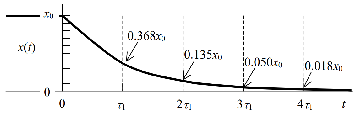
At the time constant, \(t=\tau_{1}\), the response has decayed to \(e^{-1}\) = 37% of the initial value. The other time “milestone” to which we shall often refer is \(t=4 \tau_{1}\), which we call the settling time, at which time the response has decayed to \(e^{−4}\) = 2% of the initial value. For most practical engineering purposes, this settling time is considered to be the time required for the response essentially to reach its final steady-state value, which is \(x\) = 0 in this case of IC response. Mathematically, \(x\rightarrow 0\) only as \(t \rightarrow \infty\).

If the constant \(a\) is positive, then we write IC solution Equation \(\ref{eqn:3.4}\) as \(x(t)=x_{0} e^{a t}\). The mathematical response represented by this solution is unbounded: \(x \rightarrow \infty\) as \(t \rightarrow \infty\). In reality, no engineering variable will ever become infinite: as the variable becomes large, something in the system will fail or overload, or the system will become nonlinear, or the response will be limited by a governor, etc. Even though the actual response will not become infinite, an exponentially increasing linear mathematical response such as this is usually undesirable for practical purposes; an engineering system that exhibits this kind of response is considered to be engineering system with unstable. On the other hand, a negative constant \(a\) is stable.

The time constant \(\tau_1\) is such an important quantity for stable 1^st order systems that we shall re-cast the standard 1^st order system ODE in terms of \(\tau_1\), rather than constant \(a\), using Equation \(\ref{eqn:3.5}\). Thus, rather than analyzing Equation 1.2.1, \(\dot{x}-a x=b u(t)\), hereafter we shall usually consider the following standard stable form for 1^st order systems:

\[\dot{x}+\frac{1}{\tau_{1}} x=b u(t)\label{eqn:3.7} \]

Stable step response

In Equation \(\ref{eqn:3.3}\), we set \(x_0\) = 0 and use time constant definition Equation \(\ref{eqn:3.5}\) to obtain

\[x(t)=b U \tau_{1}\left(1-e^{-t / \tau_{1}}\right) \equiv b U \tau_{1}\left[1-\exp \left(-t / \tau_{1}\right)\right], \text { for } t \geq 0\label{eqn:3.8} \]

Figure \(\PageIndex{2}\) is a graph of the exponential rise to a positive final value that is indicated in Equation \(\ref{eqn:3.8}\).

Figure \(\PageIndex{2}\): 1^st order step response

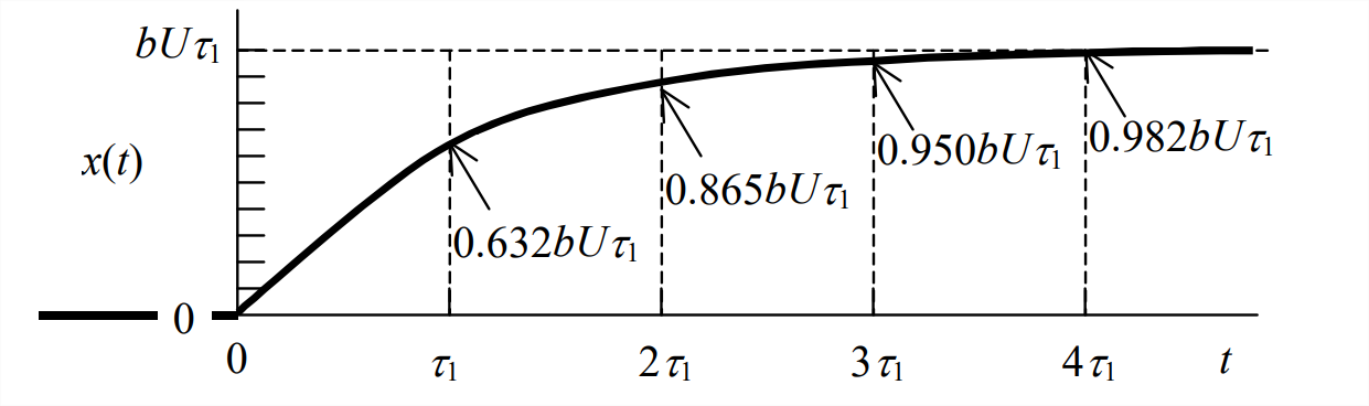
The final value of unit-step response is \(b U \tau_{1}\), and it is approached asymptotically as \(t \rightarrow \infty\). At the time constant, \(t=\tau_{1}\), the response has risen from the IC of zero to \(1-e^{-1}\) = 63%. At \(t=4 \tau_{1}\), the settling time, the response has risen to \(1-e^{-4}\) = 98% of the final value.

Step response solutions such as Equation \(\ref{eqn:3.8}\) are usually an approximation to the actual response since, in reality, a pure, discontinuous step change in a physical input quantity is rarely achievable. Nevertheless, step input is a sufficiently close approximation to many real physical inputs that step response solutions such as Equation \(\ref{eqn:3.8}\) are close approximations to actual physical responses.

Consider again the reaction wheel of the previous section. Let us denote a step input from the motor as \(M_{m}(t)=M \times H(t)\). Then ODE Equation 3.3.3 becomes

\[\dot{p}-a p=b M_{m}(t)=b M H(t)=b M \text { for } t>0, \text { where } a=-\frac{c_{\theta}}{J}=-\frac{1}{\tau_{1}} \text { and } b=\frac{1}{J}\label{eqn:3.9} \]

So the time constant is \(\tau_{1}=-1 / a=J / c_{\theta}\), and solution Equation \(\ref{eqn:3.8}\) becomes

\[p(t)=b M \tau_{1}\left(1-e^{-t / \tau_{1}}\right)=\frac{1}{J} M \frac{J}{c_{\theta}}\left(1-e^{-t / \tau_{1}}\right)=\frac{M}{c_{\theta}}\left(1-e^{-t / \tau_{1}}\right) \mathrm{rad} / \mathrm{sec}, \text { for } t \geq 0\label{eqn:3.10} \]

Note that in this case we adapt the “standard” mathematical solution Equation \(\ref{eqn:3.8}\) to a particular physical problem. This approach is common in system dynamics. In other words, it is not always necessary to solve an ODE for every new physical problem; if a standard ODE solution has already been derived, you may just adapt that standard solution to the physical problem at hand, rather than re-deriving the ODE solution.