3.5: Aileron-Induced Rolling of an Airplane or Missile

The principal source for the aerodynamic theory of this section is Nelson, 1989, pages 19-20, 153-156 and 250-260. The aerodynamic rolling moment on an airplane or missile is written in standard aeronautical notation as

\[\begin{align} L(t) &=\frac{\partial L}{\partial \delta} \delta(t)+\frac{\partial L}{\partial p} p(t) \\[4pt] &\equiv L_{\delta} \delta(t)+L_{p} p(t) \label{eqn:3.11} \end{align} \]

There is a notational ambiguity between moment \(L(t)\) and the Laplace transform operator \(L[f(t)]\) introduced in Chapter 2; such ambiguities are unavoidable in technical work, so you should become accustomed to them.

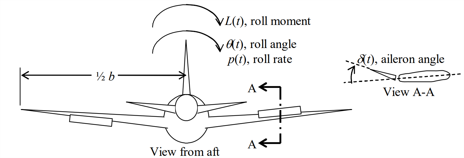
The roll (bank) angle (in radians) is \(\theta(t)\), defined here as being positive clockwise as seen by an observer behind the vehicle, in other words, rightward rolling (Figure \(\PageIndex{1}\)). In Equation \(\ref{eqn:3.11}\), \(\delta(t)\) is the input aileron deflection angle (in radians) to produce rolling, the right aileron being deflected upward and the left aileron being deflected downward to produce a positive roll rate, \(p(t) \equiv \dot{\theta}\) (rad/s).

Figure \(\PageIndex{1}\): Aileron-induced rolling of an airplane

The dimensional aerodynamic derivatives in Equation \(\ref{eqn:3.11}\) are related to dimensionless coefficients by:

\[L_{\delta}=\bar{q} S b C_{\delta}>0 \quad\left(\frac{1 b-f t}{r a d} \text { or } \frac{N-m}{r a d}\right)\label{eqn:3.12} \]

\[L_{p}=\bar{q} S b \frac{b}{2 V} C_{p}=\frac{\bar{q} S b^{2}}{2 V} C_{p}<0 \quad\left(\frac{1 \mathrm{b}-\mathrm{ft}}{\mathrm{rad} / \mathrm{sec}} \operatorname{or} \frac{\mathrm{N}-\mathrm{m}}{\mathrm{rad} / \mathrm{sec}}\right)\label{eqn:3.13} \]

The constants in Equations \(\ref{eqn:3.12}\) and \(\ref{eqn:3.13}\) are defined as:

• \(\bar{q}=\frac{1}{2} \rho V^{2}\) is the free-stream dynamic pressure (lb/ft² or N/m²)
• \(\rho\) is air density (slug/ft³ or kg/m³)
• \(V\) is the free-stream airspeed (ft/s or m/s)
• \(S\) is the wing planform area (ft² or m²)
• \(b\) is the full wing span (ft or m)
• \(C_{\delta}>0\) is the dimensionless aerodynamic stability moment coefficient (rad⁻¹), rolling moment due to aileron deflection (a function of Mach number)
• \(C_p <0\) is the dimensionless aerodynamic stability moment coefficient (rad⁻¹), roll damping due to roll rate (a function of Mach number).

The term \(b / 2 V\) in Equation \(\ref{eqn:3.13}\), the damping moment due to roll rate, merits some explanation. The clockwise rolling velocity of the right wingtip is \(p \times b / 2\), so the additional angle of attack induced at the wingtip by the roll rate is \(\tan ^{-1}\left[\frac{p b / 2}{V}\right] \approx \frac{p b}{2 V}\), a small angle (the magnitude of the angle is exaggerated in Figure \(\PageIndex{2}\), just to improve clarity). Thus, \(\frac{b}{2 V} p(t)\) in Eqsuations \(\ref{eqn:3.13}\) and \(\ref{eqn:3.11}\) plays the same role as that of \(\delta(t)\) in Eqs. \(\ref{eqn:3.12}\) and \(\ref{eqn:3.11}\).

Newton’s 2^nd law equation of motion for rolling is \(J \ddot{\theta} \equiv J \dot{p}=L(t)\), in which \(J\) (slug-ft2 or kg-m2 ) is the rotational inertia of the vehicle about its rolling axis. This equation is based upon the assumption that the vehicle can only roll (i.e., no coupling with other degrees of freedom such as sideslip and yaw). Substituting Eqs. \(\ref{eqn:3.11}\)-\(\ref{eqn:3.13}\) into Newton’s law gives:

\[J \dot{p}=L_{\delta} \delta+L_{p} p \Rightarrow J \dot{p}-L_{p} p=L_{\delta} \delta \nonumber \]

\[\Rightarrow \quad \dot{p}+\left(\frac{-L_{p}}{J}\right) p=\left(\frac{-L_{p}}{J}\right)\left(\frac{L_{\delta}}{-L_{p}}\right) \delta(t)=\left(\frac{-L_{p}}{J}\right) \frac{2 V}{b}\left(\frac{C_{\delta}}{-C_{p}}\right) \delta(t)\label{eqn:3.14} \]

Writing Equation \(\ref{eqn:3.14}\) in 1^st order standard form Equation 3.4.8 gives [with \(b\) in Equation 3.4.8 temporarily replaced by \(B\) to reduce notational ambiguity]:

\[\dot{p}+\frac{1}{\tau_{1}} p=B \delta(t)\label{eqn:3.15} \]

in which we have, respectively, time constant \(\tau_1\) and constant \(B\):

\[\tau_{1}=\frac{J}{-L_{p}}=\frac{2 V J}{\bar{q} S b^{2}\left(-C_{p}\right)}=\frac{4 J}{\rho V S b^{2}\left(-C_{p}\right)}>0\label{eqn:3.16} \]

\[B=\left(\frac{-L_{p}}{J}\right) \frac{2 V}{b}\left(\frac{C_{\delta}}{-C_{p}}\right)=\frac{1}{\tau_{1}} \frac{2 V}{b}\left(\frac{C_{\delta}}{-C_{p}}\right)=\frac{\bar{q} S b C_{\delta}}{J}>0\label{eqn:3.17} \]

Example \(\PageIndex{1}\)

Use the results of this section and the general 1^st order step response Equation 3.4.9 to calculate rolling response to a \(\delta(t)=2.5^{\circ} \mathrm{H}(t)\) step aileron input for a hypothetical medium-sized civilian transport airplane. The following are representative data: rotational inertia about the rolling axis is \(J\) = 4.0e5 slug-ft², wing planform area is \(S\) = 1 100 ft² , and wing span is \(b\) = 90 ft; for flight at 10 000 ft altitude and free-stream airspeed \(V\) = 350 ft/s, aerodynamic dimensionless rolling-moment coefficients are \(C_\delta\) = 0.061 per radian and \(C_p\) = -0.34 per radian. At 10 000 ft altitude, standard air density is \(\rho\) = 0.001 755 slug/ft³ (Nelson, 1989, p. 248).

Solution

\[\bar{q}=\frac{1}{2} \rho V^{2}=\frac{1}{2} \times 1.755 e-3 \frac{\mathrm{slug}}{\mathrm{ft}^{3}} \times\left(350 \frac{\mathrm{ft}}{\mathrm{s}}\right)^{2}=107.5 \frac{\mathrm{lb}}{\mathrm{ft}^{2}} \nonumber \]

\[L_{p}=\frac{\bar{q} S b^{2}}{2 V} C_{p}=\frac{107.5 \mathrm{lb} / \mathrm{ft}^{2} \times 1,100 \mathrm{ft}^{2} \times(90 \mathrm{ft})^{2}}{2 \times 350 \mathrm{ft} / \mathrm{s}} \times\left(-0.34 \mathrm{rad}^{-1}\right)=-4.65 \mathrm{e} 5 \frac{\mathrm{lb}-\mathrm{ft}}{\mathrm{rad} / \mathrm{s}} \nonumber \]

\[\tau_{1}=\frac{J}{-L_{p}}=\frac{4.0 \mathrm{e} 5 \mathrm{lb}-\mathrm{s}^{2}-\mathrm{ft}}{4.65 \mathrm{e} 5 \mathrm{lb}-\mathrm{s}-\mathrm{ft} / \mathrm{rad}}=0.86 \mathrm{s} \nonumber \]

(Comments regarding units: Angle is a dimensionless quantity, so the radian, which is the fundamental metric of angle, is unitless. In the calculation above for \(L_p\), all of the units shown, including radian, balance in the final result to give the correct resulting unit, \(\frac{1 \mathrm{b}-\mathrm{ft}}{\mathrm{rad} / \mathrm{s}}\); it is important to recognize this unit as opposed, for example, to \(\frac{1 b-f t}{\operatorname{deg} /s}\), which would be the case if \(C_p\) were given per degree. However, in calculations that produce results which are not angular quantities, such as \(\tau_1\) above, the radian must be recognized as unitless, and it should not appear in the units of the is final numerical result. This a general characteristic that can confuse us when we check to make certain that units of numerical answers are correct.)

\[B=\frac{1}{\tau_{1}} \frac{2 V}{b}\left(\frac{C_{\delta}}{-C_{p}}\right)=\frac{1}{0.86 \mathrm{s}} \times \frac{2 \times 350 \mathrm{ft} / \mathrm{s}}{90 \mathrm{ft}} \times \frac{0.061 \mathrm{rad}^{-1}}{0.34 \mathrm{rad}^{-1}}=1.62 \mathrm{s}^{-2} \nonumber \]

From Equation 3.4.9, the roll-rate response to the 2.5° step input is

\[p(t)=B U \tau_{1}\left[1-\exp \left(-t / \tau_{1}\right)\right]=1.62 s^{-2} \times 2.5 \operatorname{deg} \times 0.86 s \times\left(1-e^{-t /(0.86 \mathrm{s})}\right) \nonumber \]

\[p(t)=3.5[1-\exp (-1.16 t)] \frac{\text { degrees }}{s} \nonumber \]

The time constant is \(\tau_{1}\) = 0.86 s, and the steady-state roll rate of 3.5 deg/s is essentially achieved in the settling time of \(4\tau_{1}\) = 3.44 s.