Consider the reaction-wheel assembly described in Section 3.3. The rotor has been carefully machined to have rotational inertia \(J\) = 2.56e-3 lb-s2-inch. We wish to determine the viscous damping constant \(c_\theta\) of the bearings by indirect experimental measurement. We feed electric current into the motor and spin up the rotor to a high speed. Then we shut off the motor, allowing the wheel to spin down freely. With an optical tachometer, we measure the spin-down rotational speed at one instant to be 4 000 revolutions per minute (rpm). Exactly 20.0 seconds later, we measure the speed to be 1 010 rpm. From these data, calculate \(c_\theta\) in consistent lb-s-inch units.
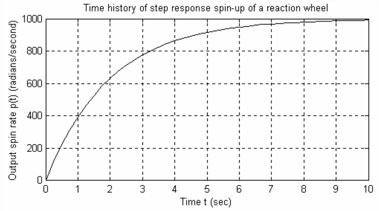
Given: an LTI reaction-wheel assembly, with unknown rotational inertia \(J\) and unknown rotational viscous damping constant \(c_\theta\) associated with drag of the bearings. Your task is to calculate \(J\) and \(c_\theta\) from experimental measurement. Starting with the wheel at rest (motionless), a motor torque in the form of a step is imposed upon the wheel, M_{m}(t)=M \times H(t), where \(M\) = 1.5 N-m. The resulting spin rate \(p(t)\) of the wheel is measured, in radians/second, and its time history for the first 10 seconds of spin-up is recorded on the following graph.
Figure \(\PageIndex{1}\)
Use the data from the graph to calculate (with as much precision as possible, given the graphical nature of the data) the values of \(J\) and \(c_\theta\) in consistent SI units.
The weight of an ocean surface ship is denoted as \(W\), and the acceleration of gravity in consistent units is \(g\). The resistance to low-velocity motion of the ship is modeled as being proportional to velocity, with viscous damping constant \(c\). The ship is initially at rest when, at time \(t\) = 0, a tugboat begins pushing it with constant force \(F\). Write algebraic equations (in terms of the given parameters, all assumed to be in consistent units) for velocity \(v(t)\) and distance traveled \(x(t)\).
Nominal data (Nelson, 1989, p. 260) for the Boeing 747 civilian transport airplane are: rotational inertia about the rolling axis \(J\) = 18.2e6 slug-ft2, wing planform area \(S\) = 5 500 ft2, and wing span \(b\) = 195.68 ft. For flight at Mach number 0.25 and at sea level altitude, nominal aerodynamic dimensionless coefficients relevant to uncoupled rolling are \(C_{\delta}\) = 0.0461 per radian and \(C_{p}\) = −0.450 per radian. At sea level, air density is \(\rho\) = 0.002377 slug/ft3, and Mach number 0.25 corresponds to free-stream airspeed \(V\) = 279.0 ft/s.
Calculate the dimensional aerodynamic derivatives \(L_{\delta}\) (in lb-ft/rad) and \(L_p\) (in lb-ft per rad/sec), then calculate the 1st order system time constant \(\tau_1\).
Suppose that the 747 is in level flight with zero initial roll rate, \(p(0)\) = 0, when the pilot cycles the ailerons through one complete sinusoid with amplitude 10° over a period of 5 seconds: \(\delta(t)=10^{\circ} \sin (0.4 \pi t)\), 0 \(\leq\) \(t\) \(\leq\) 5 s. Calculate the roll rate \(p\) (in degrees per s) at the end of the 5-second period. Do not develop any new theoretical solutions for this problem; just adapt to this problem the result of Problem 1.5.1. Your intuition might suggest that roll rate is zero at the end of the aileron cycling, since the total aileron “impulse” is zero, but you should find that roll rate is not zero.
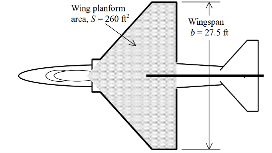
The A-4 Skyhawk was a durable and versatile small (17.5-24.5 klb) fighter-bombertrainer that first flew in 1954 and was still used in military operations, with updated technology, in the 1990s (Lightbody et al., 1990, pp. 104-111). The relevant mass and geometry data for one model are: rolling rotational inertia \(J\) = 8 090 slug-ft2; wing planform area \(S) = 260 ft2; wing span \(b\) = 27.5 ft. A flight test of this airplane is conducted at sea level and Mach number 0.4, for which the air density is \(\rho\) = 0.002377 slug/ft3 and the free-stream velocity is \(V\) = 446.6 ft/s. Starting from straight and level flight, the pilot at time \(t\) = 0 sec abruptly actuates the ailerons to +5° deflection, producing a step input that rolls the airplane clockwise. The resulting roll rate is sensed by a rate gyroscope, digitized, and recorded. The data are analyzed, and it is found that the following equation fits the data very well: \(\dot{\theta}(t)=p(t)=50.0\left(1-e^{-1.667 t}\right)\) degrees/s.
Figure \(\PageIndex{2}\): Planform sketch of A4D fighter airplane
Use the measured roll rate to perform parameter identification, specifically to determine values for the two roll aerodynamic stability coefficients \(C_\delta\) and \(C_p\), both dimensionless. Begin by calculating time constant \(\tau_1\) of the response, then use that to calculate aerodynamic derivative \(L_p\), then use that to calculate \(C_p\). Having these values, you can now use the steady-state roll rate to calculate \(C_\delta\). Check the units of your calculations to make certain that your final calculated coefficients are, in fact, dimensionless.
Given that \(\theta(0)\) = 0 (level flight), derive an equation for \(\theta(t)\) in degrees, \(t\) \(\leq\) 0. Evaluate that equation to calculate the bank angles at \(t=\tau_{1}\) (one time constant) and at \(t=4\tau_{1}\) (\(\approx\) steady-state roll rate).
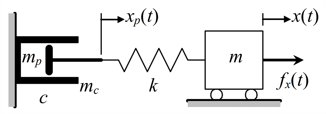
Sketch (carefully) the appropriate free-body diagrams for the mechanical system drawn below. The dashpot’s damping coefficient is \(c\), its cylinder is fixed to the wall, and its piston has mass \(m_p\). Next, use the FBDs and appropriate linear laws for the spring and dashpot to derive the ODEs that describe the motion of this system in terms of dependent variables \(x_p(t)\) and \(x(t)\). Note that the spring stretch is \(x-x_{p}\), so the tensile force developed in the spring is \(k\left(x-x_{p}\right)\). Do not neglect the inertial forces of the dashpot’s piston and of the block with mass \(m\), which rolls without friction. Force \(f_{x}(t)\) is an independent input quantity.
Figure \(\PageIndex{3}\): Series mass-dashpot-spring system
The LTI damper-spring high-pass filter of Figure 3.7.4 is repeated below. In this problem, neglect inertial forces of the damper and the spring. Input \(x_i(t)\) is translation of the damper piston, generated by some displacement-controlling motor. Output \(x_0(t)\) is translation of the damper cylinder and spring end. Sketch an appropriate free-body diagram (or more than one), then write equilibrium equation(s) from which you derive the ODE \(\tau_{1} \dot{x}_{o}+x_{o}=\tau_{1} \dot{x}_{i}\), which has right-hand-side (RHS) dynamics. Express time constant \(\tau_1\) in terms of damper constant \(c\) and spring constant \(k\). (Hint: recognize that piston force \(f_x(t)\) shown is a dependent variable, related to independent input \(x_i(t)\) and output \(x_0(t)\), but \(f_x(t)\) should not appear in the equation of motion.)