5.3: Operational Amplifier (op-amp) and Op-amp Circuits
- Page ID
- 7651

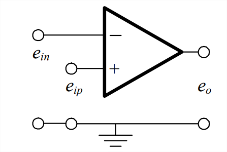
Figure \(\PageIndex{1}\) is the standard graphical symbol for an operational amplifier (op-amp). An op-amp has a “positive” input port that accepts input voltage \(e_{i p}\), and a “negative” input port that accepts input voltage \(e_{i n}\). The symbols \(e_{i p}\) and \(e_{i n}\) are merely labels; they are not meant to restrict the polarities of these input voltages, each of which can be either positive or negative relative to the ground potential. An opamp has a single output voltage, labeled \(e_{o}\) on Figure \(\PageIndex{1}\). The fundamental ideal output-to-input relationship of an op-amp is (Horowitz and Hill, 1980, Chapter 3)
\[e_{o}=K\left(e_{i p}-e_{i n}\right)\label{eqn:5.10} \]
In Equation \(\ref{eqn:5.10}\), gain \(K\) is a very large positive number, on the order of 105 to 106 for common, commercially available op-amps. The exact value of \(K\) varies gradually with the frequency of signals \(e_{i p}\) and \(e_{i n}\), but this variation is not important provided that frequency is below a known upper value; as we shall see, a very important characteristic is that \(K\) is large, \(K \geq \mathrm{O}\left(10^{5}\right)\). (This equation is a common mathematical expression meaning “\(K\) is on the order of or greater than 105.”) Another important characteristic of an op-amp is the extremely high resistance of the input ports, on the order of 106 \(\Omega\) to 1012 \(\Omega\). The practical consequence of this high resistance is that essentially zero current can flow through the input ports.
An op-amp is an active device, requiring external power to produce high gain, unlike the simple passive elements (resistor, capacitor, and inductor) of Section 5.2. An energy source (e.g., a \(\pm\)15-volt power supply, or a pair of 9-volt batteries) is usually connected to an op-amp, but this connection is normally not indicated on graphical representations such as Figure \(\PageIndex{1}\). An op-amp itself is a complex integrated circuit, full of miniaturized transistors and other electrical components. The physical form of op-amp seen most commonly on circuit boards is approximately the size and similar in appearance to a basement centipede with a black body (actually, more like a 8-legged or 16-legged insect, because it has on each side four or eight metal connectors that look like legs).
Op-amps are not often used in the open-loop configuration of Figure \(\PageIndex{1}\). Most op-amps can operate linearly according to Equation \(\ref{eqn:5.10}\) only over a limited range of \(\pm E_{l i m}\) on output voltage \(e_{o}\). The range depends upon the energy source, but typically \(E_{l i m}\) is on the order of 10 V. If the input voltages \(e_{i p}\) and \(e_{i n}\) are such that Equation \(\ref{eqn:5.10}\) leads numerically to \(e_{o}\) greater than \(+E_{l i m}\) or less than \(-E_{l i m}\), then a real op-amp will limit and stick nonlinearly on either \(+E_{l i m}\) or \(-E_{l i m}\), respectively. When this happens, the op-amp is said to be overloaded or saturated. Since gain \(K\) in Equation \(\ref{eqn:5.10}\) is so high, the input voltage difference \(e_{i p}-e_{i n}\) clearly must be very small in order for the op-amp to operate in the linear range for which it is primarily designed.
To operate an op-amp in its linear range, we almost always use feedback. When there is an electrical connection between the output port and the negative input port, the op-amp is said to be wired in a closed-loop manner, with feedback from output to input, specifically in this case, negative feedback. This negative feedback acts to make the input voltage difference \(e_{i p}-e_{i n}\) so small that for practical purposes there is no difference, \(e_{i p} \approx e_{i n}\).
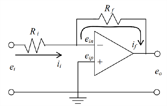
We can illustrate the practical functioning of an op-amp by analyzing in detail what is probably the most common basic circuit consisting of an op-amp and resistors, the inverting amplifier depicted in Figure \(\PageIndex{2}\). Note that there is an input resistor \(R_{i}\), and that there is negative feedback through feedback resistor \(R_{f}\). These resistances are chosen to be on the order of 101 -104 \(\Omega\), at least two orders of magnitude less than the input resistances of the op-amp ports. Note also that the positive input port is grounded, \(e_{i p}\) = 0 V. Hence, from Equation \(\ref{eqn:5.10}\),
\[e_{o}=K\left(0-e_{i n}\right) \Rightarrow e_{i n}=-\frac{e_{o}}{K}\label{eqn:5.11} \]
Due to the extremely high resistance of the negative input port relative to \(R_{i}\) and \(R_{f}\), the current through that port is essentially zero, so Kirchhoff’s current law in this case requires the feedback current to equal the input current, \(i_{i}=i_{f}\). Using Ohm’s law to write this condition of current continuity in terms of voltages gives
\[\frac{e_{i}-e_{i n}}{R_{i}}=\frac{e_{i n}-e_{o}}{R_{f}} \Rightarrow \frac{e_{i}-\left(-e_{o} / K\right)}{R_{i}}=\frac{\left(-e_{o} / K\right)-e_{o}}{R_{f}}\label{eqn:5.12} \]
With a little algebra (which you should verify on your own), the solution of Equation \(\ref{eqn:5.12}\) for circuit output voltage in terms of input voltage is found to be
\[e_{o}=-\frac{R_{f}}{R_{i}} e_{i} \frac{1}{1+\frac{1}{K}\left(1+\frac{R_{f}}{R_{i}}\right)}\label{eqn:5.13a} \]
Let us evaluate the denominator of the large fraction in Equation \(\ref{eqn:5.13a}\). In typical applications of this circuit, the resistance ratio \(R_{f} / R_{i}\) is on the order of 102 at most. Therefore, with gain \(K=\mathrm{O}\left(10^{5}\right)\), the denominator is very, very close to 1: \(1+\mathrm{O}\left(10^{-3}\right) \approx 1\). (This validates the earlier statement that only the large magnitude of \(K\) matters, the exact value being unimportant.) So, the entire large fraction is essentially equal to one, and Equation \(\ref{eqn:5.13a}\) simplifies considerably to
\[e_{o}=-\frac{R_{f}}{R_{i}} e_{i}\label{eqn:5.13b} \]
The output voltage equals the input voltage amplified by the ratio \(R_{f} / R_{i}\), and the sign is inverted; hence the name inverting amplifier.
Note also, from Equation \(\ref{eqn:5.11}\), that the voltage at the negative input port is negligibly small relative to the output (and input) voltages:
\[e_{i n}=-\frac{e_{o}}{K} \approx 0=e_{i p}(\text { the voltage of the grounded port })\label{eqn:5.14} \]
In other words, the op-amp’s high gain drives the voltage \(e_{i n}\) at the negative input port to be essentially equal to the voltage \(e_{i p}\) at the positive input port. Equation \(\ref{eqn:5.14}\) is just a special case of the simplifying assumption that we can use in general, from Equation \(\ref{eqn:5.10}\),
\[e_{i p}-e_{i n}=\frac{e_{o}}{K} \approx 0 \Rightarrow e_{i n}=e_{i p}\label{eqn:5.15} \]
In circuit analysis, Equation \(\ref{eqn:5.15}\) is considered a useful “rule” or “axiom” rather than just an assumption. In the future (unless directed otherwise, as for a homework or exam problem), you should always apply rule Equation \(\ref{eqn:5.15}\) right from the very beginning of the derivation for an op-amp circuit with negative feedback, because it simplifies the derivation so much. For example, if we use Equation \(\ref{eqn:5.15}\) from the beginning for the inverting amplifier, then the derivation becomes two easy steps [using \(e_{i n}=e_{i p}=0\) in Equation \(\ref{eqn:5.12}\)]:
\[\frac{e_{i}-0}{R_{i}}=\frac{0-e_{o}}{R_{f}} \Rightarrow e_{o}=-\frac{R_{f}}{R_{i}} e_{i} \nonumber \]
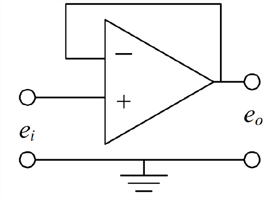
Figure \(\PageIndex{3}\) depicts an extremely simple, closed-loop op-amp circuit that is useful in practice. The input voltage signal is directed into the positive input port, and this port’s high resistance prevents the flow of any current from the input source. Equation \(\ref{eqn:5.15}\) in combination with the feedback connection states that the output voltage exactly equals the input voltage, \(e_{o}=e_{i}\). This op-amp circuit functions as a current isolator and voltage transmitter, and it is usually called a voltage follower. Its main value is in providing a buffer between two different stages of a more complex circuit: the buffer allows the output voltage of the upstream stage to be the input voltage of the downstream stage, without permitting any current flow between the two stages. Any such interstage current flow would usually cause malfunctioning of both stages. The application of a voltage follower as a buffer between circuit stages is illustrated in the next section.