5.5: Chapter 5 Homework

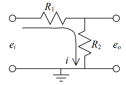
1. The simple series circuit represented graphically below is a voltage divider, which is widely used in practical applications. Show that the voltage output-to-input ratio is \[\frac{e_{o}}{e_{i}}=\frac{R_{2}}{R_{1}+R_{2}} \nonumber \]

   

2. Two capacitors are arranged in series, as shown below.

   

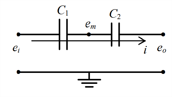
   1. Use the current-voltage equation for capacitor \(C_1\) to show that \(\dot{e}_{m}=\dot{e}_{i}-\frac{i}{C_{1}}\), where the \(e\)'s are the voltages indicated on the drawing and \(i\) is the current.
   2. Use the result of part 5.2.1 and the capacitor current-voltage equation for capacitor \(C_2\) in order to derive an algebraic formula for the equivalent series capacitance \(C_{e q}\) (in terms of \(C_1\) and \(C_2\)) in the equation \(i=C_{e q}\left(\dot{e}_{i}-\dot{e}_{o}\right)\).
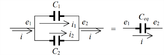
3. Given capacitors \(C_1\) and \(C_2\) arranged in parallel, as shown below, find the equivalent single capacitance \(C_{e q}\).

   

4. The simple circuit represented graphically below is a 1^st order RC high-pass filter.

   

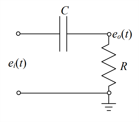
   1. Use current continuity and the formulas relating current to voltage-difference for resistors and capacitors to derive in all detail the following ODE with right-hand-side (RHS) dynamics, which governs the output voltage \(e_{o}(t)\) in terms of input voltage \(e_{i}(t)\): \[\dot{e}_{o}+\frac{1}{\tau_{1}} e_{o}=\dot{e}_{i}, \tau_{1}=R C \nonumber \] Explain why this circuit is considered to be an exact electrical analog of the mechanical series damper-spring high-pass filter described in Figure 3.7.4 and Equation 3.7.6.
   2. For frequency response, the input voltage is \(e_{i}(t)=E_{i} \cos \omega t\) and the steady-state output voltage is \(e_{o}(t)=E_{o} \cos (\omega t+\phi)\). Use the governing equation from part 5.4.1 to derive the algebraic equations for FRF of the 1^st order high-pass filter: the magnitude ratio \(E_{o}(\omega) / E_{i}\) and the phase \(\phi(\omega)\) (in radians) as functions of excitation frequency \(\omega\). (partial answer: \(E_{o}(\omega) / E_{i}=\omega \tau_{1} / \sqrt{1+\left(\omega \tau_{1}\right)^{2}}\).) Suppose that \(R\) = 40 k\(\Omega\) and \(C\) = 0.25 \(\mu\)F (recall that \(\mu\) = 10^-6). Calculate the break frequency \(f_{b}=1 /\left(2 \pi \tau_{1}\right)\) in Hz. To get some feeling for the functioning of a high-pass filter, calculate the FRF magnitude ratio \(E_{o}(\omega) / E_{i}\) for driving frequency ratios \(f / f_{b}\) = 0.01, 0.1, 1, 10, and 100. (See also homework Problem 4.4.)
   3. Suppose that the input voltage is a ramp, \(e_{i}(t)=e_{r}\left(t / t_{r}\right) H(t)\), where \(e_{r}\) is a reference voltage and \(t_{r}\) is a reference time such that \(e_{i}\left(t_{r}\right)=e_{r}\). For IC \(e_{o}(0)\) = 0 volt, solve the governing ODE from part 5.4.1 for the algebraic equation for \(e_{o}(t)\) in terms of the given algebraic parameters. Note that the derivative of the input voltage in this case is a step function, \(\dot{e}_{i}(t)=\left(e_{r} / t_{r}\right) H(t)\).
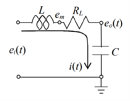
5. The circuit drawn below is a series combination of a voltage source \(e_{i}(t)\), a coil (having both inductance \(L\) and resistance \(R_L\)), and a capacitor \(C\); this is known as an \(LRC\) circuit. The input voltage is applied at time \(t\) = 0, at which time there is a non-zero voltage on the capacitor, . Apply Kirchhoff’s voltage law, as in Electricity Example 5.2.4, and show that the equation for current \(i(t) \text { is } L \frac{d i}{d t}+R_{L} i+\frac{1}{C} \int_{\tau=0}^{\tau=t} i(\tau) d \tau=e_{i}(t)-e_{o}(0)\).

   

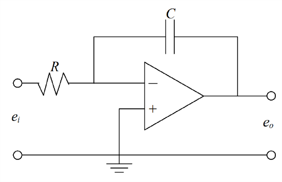
6. For the op-amp circuit represented graphically at right, an integrator, derive the algebraic equation for the transfer function between input and output voltages, \(T F(s)=\frac{L\left[e_{o}(t)\right]}{L\left[e_{i}(t)\right]}\). Assume that there is no initial charge on the capacitor at time \(t\) = 0. To simplify the derivation, apply rule Equation 5.3.7.¹

   

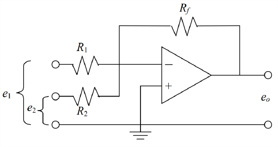
7. For the op-amp circuit represented graphically below, a summing inverting amplifier, derive the algebraic equation for output voltage \(e_{o}(t)\) in terms of resistances \(R_1\), \(R_2\), and \(R_f\), and input voltages \(e_1(t)\) and \(e_2(t)\). To simplify the derivation, apply rule Equation 5.3.7.

   

8. 1. For the op-amp circuit represented graphically below, a non-inverting amplifier, derive the algebraic equation for output voltage \(e_{o}(t)\) in terms of resistances \(R_1\) and \(R_2\), and input voltage \(e_{i}(t)\). To simplify the derivation, apply rule Equation 5.3.7.

      

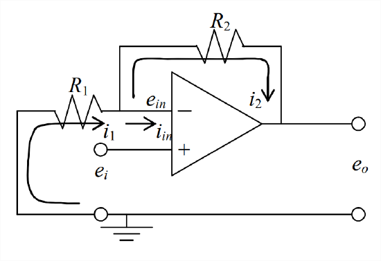
   2. Suppose that \(e_{i}\) = 1.6 V, \(R_1\) = 5 k\(\Omega\), and \(R_2\) = 15 k\(\Omega\). Determine the values of \(e_{i n}\) (in V), \(i_{i n}\) (in milliamps, mA), \(i_1\) (in mA), \(i_2\) (in mA), and \(e_o\) (in V).
9. The circuit drawing below shows an inverting amplifier, from Figure 5.3.2, and, at the input of the amplifier, a variable resistor with a sliding contact, often called a wiper. The maximum useable resistance of the variable resistor is \(R_p\); however, by moving the wiper along the surface of the resistor (adjusted by turning a dial or a screw), we can connect between \(e_{i}\) and \(e_{i m}\) any portion \(\alpha R_{p}\), where \(0 \leq \alpha \leq 1\). The purpose of this particular circuit configuration is to allow the gain constant of the amplifier to adjusted continuously to any value between zero and \(R_{f} / R_{i}\), rather than being constrained to the value \(R_{f} / R_{i}\) of Equation 5.3.5. Your assignment is to derive the following voltage output-to-input equations: \[\frac{e_{i m}}{e_{i}}=\frac{(1-\alpha)}{1+\alpha(1-\alpha) \frac{R_{p}}{R_{i}}} \Rightarrow \frac{e_{o}}{e_{i}}=-\frac{(1-\alpha) \frac{R_{f}}{R_{i}}}{1+\alpha(1-\alpha) \frac{R_{p}}{R_{i}}} \nonumber \] In your derivation, do not neglect the current to ground through the side of the variable resistor with resistance \((1-\alpha) R_{p}\). For applications in electronic analog computers (see the footnote to homework Problem 5.6), this arrangement of a variable resistor is called a coefficient-setting potentiometer or just a pot for short.

   

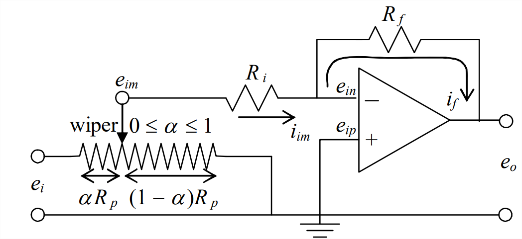
   Inverting amplifier with coefficient-setting potentiometer

10. The circuit represented graphically below consists of two stages, each stage being built around an op-amp.

    

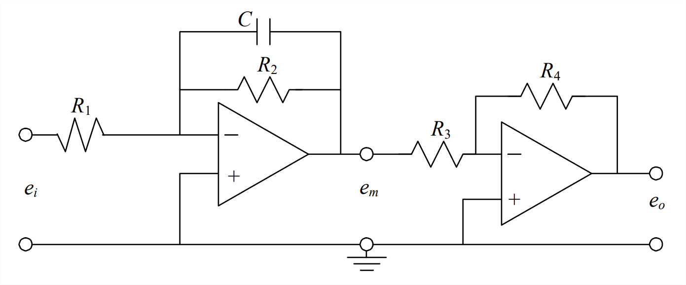
    1. Derive from the left-hand stage the following ODE for interstage voltage \(e_{m}(t)\): \[\dot{e}_{m}+\frac{1}{R_{2} C} e_{m}=-\frac{1}{R_{1} C} e_{i} \nonumber \]
    2. Combine the result of part 5.10.1 with the effect of the right-hand stage to show that the ODE for output voltage \(e_{o}(t)\) is \(\dot{e}_{o}+\frac{1}{R_{2} C} e_{o}=\frac{R_{4}}{R_{3}} \frac{1}{R_{1} C} e_{i}\). (Note: This circuit is essentially the electronic analog computer (see the footnote to homework Problem 5.6) for solving the standard stable 1^st order ODE Equation 3.4.8, \(\dot{x}+\left(1 / \tau_{1}\right) x=b u(t)\). Input voltage \(e_{i}(t)\) is analogous to standard input \(u(t)\), output voltage \(e_{o}(t)\) is analogous to response , time constant \(\tau_{1}=R_{2} C\), and constant \(b=\frac{R_{4}}{R_{3}} \frac{1}{R_{1} C}\).)
11. The circuit represented graphically on the next page is the basic, ideal form of electronic analog proportional-integral (PI) controller, one of the subjects of Chapter 15. (In practice, a great deal of electronic refinement and conditioning is required to produce a circuit that behaves even close to ideally.) The input voltage signal is \(e_{e}(t)\), the intermediate voltage between the two stages is \(e_{m}(t)\), and the output voltage from the PI controller is \(w(t)\).

    

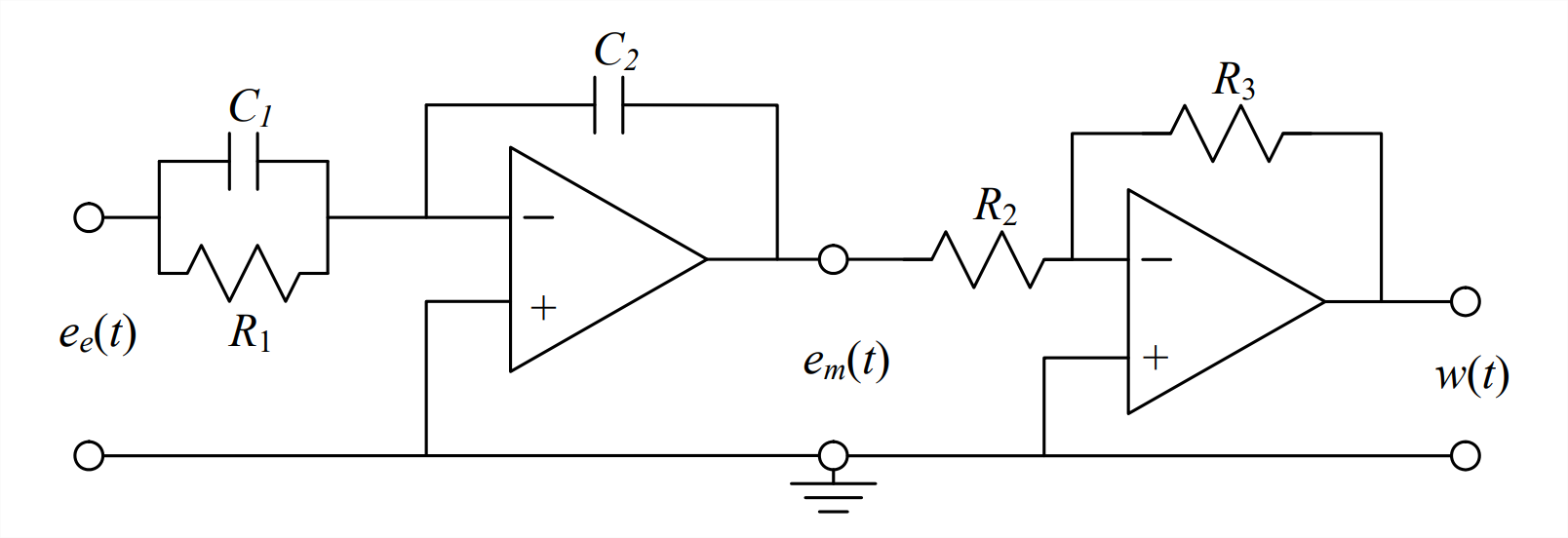
    1. By applying the methods of circuit analysis described in Chapter 5, show that the ODE relating PI-controller output \(w(t)\) to input \(e_{e}(t)\), expressed in terms of the capacitor and resistor parameters of the circuit diagram, is: \[\dot{w}=\frac{R_{3} C_{1}}{R_{2} C_{2}}\left(\dot{e}_{e}+\frac{1}{R_{1} C_{1}} e_{e}\right) \nonumber \]
    2. Derive the PI-controller transfer function \(T F(s) \equiv \frac{\left.L[w(t)]\right|_{w_{0}=0}}{\left.L\left[e_{e}(t)\right]\right|_{e_{e}=0}}\), expressed in terms of the capacitor and resistor parameters of the circuit diagram.

¹This integrator seems simple on paper, but design of a real integrator that functions properly is difficult, requiring expensive, precision components and many subtle refinements of the basic circuit. Integrators based upon this circuit are essential components of the electronic analog computer (EAC), an elegant instrument dating from the 1940s for solving coupled ODEs, but one that has now almost completely been replaced by digital computers. Fifer’s 1961 four-volume set is probably the most complete description of all types of analog computers; Peterson’s 1967 textbook includes standard instructional material on EACs; and Lang’s 2000 article is an interesting, more modern discussion of EACs.