6.3: Examples of First Order System Response

Example \(\PageIndex{1}\)

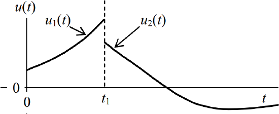
It is often the case that the input to a system is described by different functions, each function in effect over a different time period for \(t > 0\). For example, the following equation and drawing represent an input consisting of two different general functions:

\[u(t)=\left\{\begin{array}{c}
0, \quad t<0 \\
u_{1}(t), \quad 0<t<t_{1} \\
u_{2}(t), \quad t_{1}<t
\end{array}\right. \nonumber \]

Solution

The general forced response to this type of input can be expressed nicely in terms of convolution integrals, but we must recognize that it requires two different equations, and we must consider carefully the limits of the definite integrals. First, for the time interval \(0 \leq t \leq t_{1}\), it is clear that the second form of Equations 6.2.4 is directly applicable, with \(u(t) \equiv u_{1}(t)\):

\[x(t)=x_{0} e^{-t / \tau_{1}}+b \int_{\tau=0}^{\tau=t} e^{-(t-\tau) / \tau_{1}} u_{1}(\tau) d \tau \quad, \text { for } 0 \leq t \leq t_{1}\label{eqn:6.6a} \]

For the response during the second time interval, \(t \geq t_{1}\), the definite integral in the second form of Equations 6.2.4 still must be evaluated over the limits \(\tau=0\) to \(\tau=t>t_{1}\), which means that both \(u_{1}\) and \(u_{2}\) need to be integrated, but each only over the time interval for which it is defined:

\[x(t)=x_{0} e^{-t / \tau_{1}}+b\left[\int_{\tau=0}^{\tau=t_{1}} e^{-(t-\tau) / \tau_{1}} u_{1}(\tau) d \tau+\int_{\tau=t_{1}}^{\tau=t} e^{-(t-\tau) / \tau_{1}} u_{2}(\tau) d \tau\right] \quad, \text { for } t \geq t_{1}\label{eqn:6.6b} \]

Note especially in Equation \(\ref{eqn:6.6b}\) that \(\tau=t_{1}\) is both the upper limit of the integral that involves \(u_1\) and the lower limit of the integral that involves \(u_2\). Equations \(\ref{eqn:6.6a}\) and \(\ref{eqn:6.6b}\) are especially useful for response to a pulse of limited duration, as is illustrated in the next example.

Example \(\PageIndex{2}\)

We consider again the problem for velocity of a mass moving on a viscous film, which is solved by basic ODE methods in Section 1.5:

\[\mathrm{ODE}+\mathrm{IC}: m \dot{v}+c v=f_{x}(t), \quad v(0)=v_{0}, \quad \text { find } v(t) \text { for } t>0\label{eqn:6.7} \]

\[f_{x}(t)=\left\{\begin{array}{c}
F \sin \left(\pi t / t_{d}\right) \equiv F \sin \omega t \quad \text { where } \omega=\pi / t_{d}, 0 \leq t \leq t_{d} \\
0, t_{d}<t
\end{array}\right. \nonumber \]

Solution

Here we have \(u(t)=f_{x}(t)\), \(\tau_{1}=m / c\), and \(b=1 / m\). Relative to the notation of Example \(\PageIndex{1}\) above, \(u_{1}\) is the half-sine pulse, and \(u_{2}\) is zero.

While the pulse is active, \(0 \leq t \leq t_{d}\), Equation \(\ref{eqn:6.6a}\) becomes

\[v(t)=v_{0} e^{-t / \tau_{1}}+\frac{F}{m} e^{-t / \tau_{1}} \int_{\tau=0}^{\tau=t} e^{\tau / \tau_{1}} \sin \omega \tau d \tau\label{eqn:6.8} \]

We can evaluate the definite integral by several different methods: find it in a table of definite integrals (or indefinite integrals, but do not forget the lower limit of integration); or integrate by parts twice; or evaluate it with software that does symbolic manipulation, such as Mathematica or recent versions of MATLAB. The result is

\[\int_{\tau=0}^{\tau=t} e^{\tau / \tau_{\mathrm{t}}} \sin \omega \tau d \tau=\frac{\tau_{1}}{1+\left(\omega \tau_{1}\right)^{2}}\left[e^{t / \tau_{1}}\left(\sin \omega t-\omega \tau_{1} \cos \omega t\right)+\omega \tau_{1}\right]\label{eqn:6.9} \]

Combining Equation \(\ref{eqn:6.8}\) and Equation \(\ref{eqn:6.9}\) gives the velocity during the pulse duration:

\[v(t)=\left[v_{0}+\frac{F}{c} \frac{\omega \tau_{1}}{1+\left(\omega \tau_{1}\right)^{2}}\right] e^{-t / \tau_{1}}+\frac{F}{c} \frac{1}{1+\left(\omega \tau_{1}\right)^{2}}\left(\sin \omega t-\omega \tau_{1} \cos \omega t\right), 0 \leq t \leq t_{d}\label{eqn:6.10} \]

At the instant \(t=t_{d}\) when the pulse goes to zero, \(\omega t_{d}=\pi\), so the velocity then is

\[v\left(t_{d}\right)=\left[v_{0}+\frac{F}{c} \frac{\omega \tau_{1}}{1+\left(\omega \tau_{1}\right)^{2}}\right] e^{-t_{d} / \tau_{1}}+\frac{F}{c} \frac{\omega \tau_{1}}{1+\left(\omega \tau_{1}\right)^{2}}\label{eqn:6.11} \]

For the time after the pulse goes to zero, \(t_{d} \leq t\), Equation \(\ref{eqn:6.6b}\) becomes

\[v(t)=v_{0} e^{-t / \tau_{1}}+\frac{F}{m} e^{-t / \tau_{1}}\left(\int_{\tau=0}^{\tau=t_{d}} e^{\tau / \tau_{1}} \sin \omega \tau d \tau+\int_{\tau=t_{d}}^{\tau=t} e^{\tau / \tau_{1}} \times 0 d \tau\right)\label{eqn:6.12} \]

With use again of Equation \(\ref{eqn:6.9}\), and of some algebra, Equation \(\ref{eqn:6.12}\) becomes

\[v(t)=v_{0} e^{-t / \tau_{1}}+\frac{F}{c} e^{-t / \tau_{1}} \frac{\omega \tau_{1}}{1+\left(\omega \tau_{1}\right)^{2}}\left(1+e^{t_{d} / \tau_{1}}\right)=v\left(t_{d}\right) e^{-\left(t-t_{d}\right) / \tau_{1}}, \text { for } t \geq t_{d}\label{eqn:6.13} \]

The final form on the right-hand side of Equation \(\ref{eqn:6.13}\) uses Equation \(\ref{eqn:6.11}\), and it shows that the post-pulse response is a pure exponential decay, which we would expect physically.

Example \(\PageIndex{3}\)

From Section 3.3, we have the equation of motion for spin velocity \(p(t)\) of a reaction wheel Figure 3.3.1 with rotational inertia \(J\), bearing viscous damping constant \(c_{\theta}\), and applied motor torque \(M_{m}(t)\):

\[\dot{p}+\frac{c_{\theta}}{J} p=\frac{1}{J} M_{m}(t) \Rightarrow \dot{p}+\frac{1}{\tau_{1}} p=b M_{m}(t) \text { where } \tau_{1}=\frac{J}{c_{\theta}} \text { and } b=\frac{1}{J} \nonumber \]

Solution

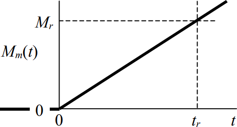
Let the initial velocity be zero, \(p(0) \equiv p_{0}=0\). Let the motor torque have the form of a ramp:

\[M_{m}(t)=\frac{M_{r}}{t_{r}} t, t \geq 0 \nonumber \]

Then the second form of general solution Equations 6.2.4 becomes

\[p(t)=p_{0} e^{-t / \tau_{1}}+b \int_{\tau=0}^{\tau=t} e^{-(t-\tau) / \tau_{1}} M_{m}(\tau) d \tau=\frac{1}{J} \int_{\tau=0}^{\tau=t} e^{-(t-\tau) / \tau_{1}} \frac{M_{r}}{t_{r}} \tau d \tau \nonumber \]

\[\Rightarrow \quad p(t)=\frac{1}{J} \frac{M_{r}}{t_{r}} e^{-t / \tau_{1}} \int_{\tau=0}^{\tau=t} e^{\tau / \tau_{1}} \tau d \tau \nonumber \]

We can evaluate the integral easily using integration by parts:

\[\int_{\tau=0}^{\tau=t} \overbrace{\tau}^{u} \overbrace{e^{\tau / \tau_{1}}}^{d v} d \tau=\left[\tau \times \tau_{1} e^{\tau / \tau_{1}}\right]_{\tau=0}^{\tau=t}-\int_{\tau=0}^{\tau=t} \tau_{1} e^{\tau / \tau_{1}} d \tau=\tau_{1} t e^{t / \tau_{1}}-\tau_{1}^{2}\left(e^{t / \tau_{1}}-1\right) \nonumber \]

Therefore, the total solution is

\[p(t)=\frac{1}{J} \frac{M_{r}}{t_{r}} e^{-t / \tau_{1}}\left[\tau_{1} t e^{t / \tau_{1}}-\tau_{1}^{2}\left(e^{t / \tau_{1}}-1\right)\right]=\frac{M_{r}}{c_{\theta} t_{r}}\left[t-\tau_{1}\left(1-e^{-t / \tau_{1}}\right)\right]\label{eqn:6.14} \]

By sketching a plot versus time of the dimensionless spin velocity \(\frac{p(t)}{M_{r} / c_{\theta}}\), you can easily show that, as \(t \rightarrow \infty\), this quantity is asymptotic to the ramp function \(\left(t-\tau_{1}\right) / t_{r}\).