6.5: Numerical Algorithm for the General Solution of the Standard First Order Problem

We seek solutions of Equation 6.4.5 in time-series form, that is, at discrete, equally spaced instants in time. Accordingly, we define the following notation that employs descriptive subscripts:

\(t=\)	\(t_1\)	\(t_{2}=t_{1}+\Delta t\)	\(t_{3}=t_{2}+\Delta t\)	\(\dots\)	\(t_{n}=t_{n-1}+\Delta t\)	\(t_{n+1}=t_{n}+\Delta t\)	\(\dots\)
\(x(t)=\)	\(x_1\)	\(x_2\)	\(x_3\)	\(\dots\)	\(x_{n}\)	\(x_{n+1}\)	\(\dots\)
\(u(t)=\)	\(u_1\)	\(u_2\)	\(u_3\)	\(\dots\)	\(u_{n}\)	\(u_{n+1}\)	\(\dots\)

Conceptually, we begin with the known values at \(t = t_1\), then integrate Equation 6.4.5 from \(t_{1}\) to \(t_{2}=t_{1}+\Delta t\), in which we define \(\Delta t\) as the constant time step; we now have known values at \(t=t_{2}\), so we can integrate again to go from \(t_{2}\) to \(t_{3}=t_{2}+\Delta t\). We proceed in this manner from one time to the next until we have determined values of \(x(t)\) at discrete instants in time over the complete time interval of interest. From Equation 6.4.5, the exact, general equation for stepping from time instant \(t_{n-1}\) to the next instant \(t_n\) is

\[x_{n}=e^{a\left(t_{n}-t_{n-1}\right)} x_{n-1}+\int_{\tau=t_{n-1}}^{\tau=t_{n}} e^{a\left(t_{n}-\tau\right)} b u(\tau) d \tau\label{eqn:6.18} \]

By comparing Equation \(\ref{eqn:6.18}\) with Equation 6.2.4, observe that the integral in Equation \(\ref{eqn:6.18}\) is clearly a forced-response convolution integral.

Up to this point, the solution is exact. But now we introduce what, in general, is an approximation. We assume that \(u(\tau)\) varies so little over the integration time step \(\Delta t\) that it introduces only small error to approximate \(u(\tau)\) as being constant over \(\Delta t\), with its value remaining that at the beginning of the integration time:

\[u(\tau) \approx u\left(t_{n-1}\right) \equiv u_{n-1} \text { for } t_{n-1} \leq \tau<t_{n}\label{eqn:6.19} \]

Using approximation Equation \(\ref{eqn:6.19}\) and \(t_{n}=t_{n-1}+\Delta t\), we rewrite Equation \(\ref{eqn:6.18}\) with the convolution integral expressed in a more easily integrable form:

\[x_{n}=e^{a \Delta t} x_{n-1}+\left[\int_{\tau=t_{n-1}}^{\tau=t_{n-1}-\Delta t} e^{a\left(t_{n-1}+\Delta t-\tau\right)} d \tau\right] b u_{n-1} \nonumber \]

We change the variable of integration, \(\xi=t_{n-1}+\Delta t-\tau\), so that the integral becomes

\[\int_{\xi=\Delta t}^{\xi=0} e^{a \xi}(-d \xi)=\int_{\xi=0}^{\xi=\Delta t} e^{a \xi} d \xi=\frac{1}{a}\left(e^{a \Delta t}-1\right) \nonumber \]

Finally, with approximation Equation \(\ref{eqn:6.19}\), solution Equation \(\ref{eqn:6.18}\) can be written as

\[x_{n}=e^{a \Delta t} x_{n-1}+\frac{1}{a}\left(e^{a \Delta t}-1\right) b u_{n-1} \equiv \phi x_{n-1}+\gamma u_{n-1}\label{eqn:6.20} \]

Equation \(\ref{eqn:6.20}\) is a recurrence formula that is easy to evaluate numerically from one time instant to the next, especially since coefficients \(\phi \equiv e^{a \Delta t}\) and \(\gamma \equiv\left(e^{a \Delta t}-1\right) b / a=(\phi-1) b / a\) are invariant once \(\Delta t\) has been selected. Note that if the input \(u(t)\) is a constant, as for a step function, then \(u_{n}=\) constant for all \(n=1,2, \ldots\), in which case Equation \(\ref{eqn:6.20}\) is an exact solution because Equation \(\ref{eqn:6.19}\) is exact, not an approximation. Furthermore, if the actual \(u(t)\) is piecewise-constant, then Equation \(\ref{eqn:6.20}\) can be applied to produce exact results, provided that \(\Delta t\) is chosen individually for each interval of constant \(u(t)\) such that the interval is an integer multiple of its own \(\Delta t\).

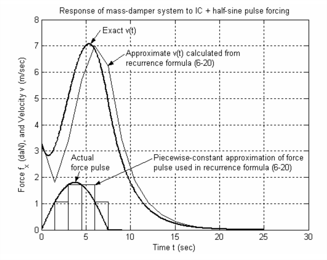
To illustrate the application of Equation \(\ref{eqn:6.20}\), we re-visit the numerical solution of Section 1.6, the velocity response of a mass-damper system to a half-sine force pulse. M-file MATLABdemo11.m of Section 1.6, which calculates the response exactly, provides the benchmark for evaluating the approximate response calculation. The MATLAB script M-file to calculate and graph the approximate response is:

%MATLABdemo61.m

%Mass-damper system approximate response to IC + half-sine pulse forcing

m=5;c=2; %system mass & viscous damping coefficient, SI units

a=-c/m;b=1/m;

F=18;td=7.5; %half-sine pulse, amplitude (N), pulse duration (s)

w=pi/td; %circular frequency of half-sine pulse (rad/s)

Dt=1.5; %time step for recurrence calculations

t=0:Dt:24;Lt=length(t); %array of time instants for recurrence calculations

phi=exp(a*Dt);gam=(phi-1)/a*b; %constants in recurrence formula

for n=1:Lt %time series array of input force pulse

if t(n)<=7.5

fx(n)=F*sin(pi*t(n)/td);

else

fx(n)=0;

end

end

v=zeros(1,Lt);v(1)=3.3; %initialize velocity array, initial velocity (m/s)

for n=2:Lt

v(n)=phi*v(n-1)+gam*fx(n-1);

end

plot(t,v,'k'),bar(t+Dt/2,fx/10,1,'k')

Note that the implementation of recurrence formula Equation \(\ref{eqn:6.20}\) in MATLABdemo61.m is a simple three-line for-loop.

The figure on the next page was produced by combining the results of M-files MATLABdemo11.m and MATLABdemo61.m, and then adding explanatory labels and editing the bar graph. For this example, time step \(\Delta t\) was intentionally chosen to be unreasonably large, \(\Delta t\) = 1.5 s (compared with system time constant \(\tau_{1}\) = 2.5 s), in order to produce clear distinctions between the exact and approximate dynamic variables. Nevertheless, the approximate calculation of velocity shows the correct trends qualitatively and is not highly inaccurate quantitatively. If the calculations were repeated with a more reasonable time step, \(\Delta t \leq 0.1 \tau_{1}\), then the results would be much more accurate (homework Problem 6.4).

Observe also in the figure on the next page the bar graph of approximate force \(f_{x}(t)\) used in Equation \(\ref{eqn:6.20}\), which is the graphical representation of approximation Equation \(\ref{eqn:6.19}\). Because of its piecewise-constant character, this is sometimes called a stairstep approximation. This approximation introduces a time delay or lag on the order of \(\Delta t\) into the approximate input. This artificial time delay is obviously transmitted to the calculated approximate response.

Figure \(\PageIndex{1}\)

It is interesting and possibly useful to observe that, due to approximating \(u(\tau)\) as being constant over each time step \(\Delta t\), Equation \(\ref{eqn:6.20}\) is essentially IC + step response over each \(\Delta t\). Suppose that we were to seek an even more accurate recurrence formula than Equation \(\ref{eqn:6.20}\) by approximating \(u(\tau)\) as varying linearly with time over each time step. In that case, the solution would be essentially IC + step response + ramp response over each \(\Delta t\). (Example 6.3 in Section 6.3 illustrates ramp response.) So the more refined approximate recurrence formula would be Equation \(\ref{eqn:6.20}\) supplemented with an additional term that represents ramp response, and we would expect that additional term to include both \(u_{n-1}\) and \(u_{n}\) as a consequence of the approximated linear variation of \(u(\tau)\); see homework Problem 6.5.