8.1: Flat Pulse

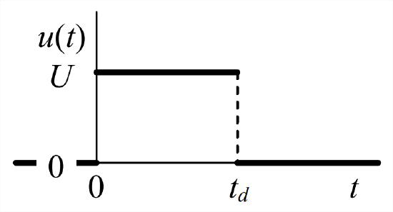
This is probably the simplest form of limited-duration input. We define the flat pulse initially in the form of a general (standard) input quantity \(u(t)\) that can be used with standard forms of system ODEs such as \(\dot{x}+\left(1 / \tau_{1}\right) x=b u(t)\) for a stable 1^st order system and \(\ddot{x}+2 \zeta \omega_{n} \dot{x}+\omega_{n}^{2} x=\omega_{n}^{2} u(t)\) for 2^nd order systems. Figure \(\PageIndex{1}\) illustrates a flat pulse of duration \(t_d\). It can be described mathematically with use of two unit-step functions, as defined in Section 2.4:

\[u(t)=U\left[H(t)-H\left(t-t_{d}\right)\right]\label{eqn:8.1} \]

The Laplace transform of Equation \(\ref{eqn:8.1}\), from Equations 2.4.4 and 2.4.5, is

\[L[u(t)]=U\left(\frac{1}{s}-\frac{e^{-s t_{d}}}{s}\right)=\frac{U}{s}\left(1-e^{-s t_{d}}\right)\label{eqn:8.2} \]

Figure \(\PageIndex{1}\): Flat pulse

Example \(\PageIndex{1}\): Response to a Flat Pulse of an Undamped 2^nd Order System¹

The ODE for an undamped 2^nd order system is \(\ddot{x}+\omega_{n}^{2} x=\omega_{n}^{2} u(t)\). Let the initial conditions be zero: \(x_{0}=0\), \(\dot{x}_{0}=0\). The general solution then is either of the two convolution integral forms, Equations 7.2.4 and 7.2.5. Of those two, the easier one to interpret for the discontinuous flat pulse is Equation 7.2.5, which with zero ICs becomes

\[x(t)=\omega_{n} \int_{\tau=0}^{\tau=t} \sin \omega_{n}(t-\tau) \times u(\tau) d \tau\label{eqn:8.3} \]

Rather than use Equation \(\ref{eqn:8.1}\) explicitly, we can observe the form of Figure \(\PageIndex{1}\) and write Equation \(\ref{eqn:8.3}\) for two different time intervals:

\[x(t)=\left\{\begin{array}{c}
\omega_{n} \int_{\tau=0}^{\tau=t} \sin \omega_{n}(t-\tau) \times U d \tau, \quad 0 \leq t \leq t_{d} \\
\omega_{n} \int_{\tau=0}^{\tau=t_{d}} \sin \omega_{n}(t-\tau) \times U d \tau+\omega_{n} \int_{\tau=t_{d}}^{\tau=t} \sin \omega_{n}(t-\tau) \times 0 d \tau, \quad t_{d} \leq t
\end{array}\right.\label{eqn:8.4} \]

The second integral for \(t_{d} \leq t\) is obviously zero. This leaves us with a single integral for each time interval, each integral having the same integrand and lower limit. However, the integrals have different upper limits, so let us denote a general upper limit as \(T\), and evaluate that common integral with use of the change of integration variable \(\lambda=t-\tau \Rightarrow d \lambda=-d \tau\):

\[\int_{\tau=0}^{\tau=T} \sin \omega_{n}(t-\tau) d \tau=\int_{\lambda=t}^{\lambda=t-T} \sin \omega_{n} \lambda(-d \lambda)=\frac{1}{\omega_{n}} \int_{\lambda=t}^{\lambda=t-T} d\left(\cos \omega_{n} \lambda\right)=\frac{1}{\omega_{n}}\left[\cos \omega_{n}(t-T)-\cos \omega_{n} t\right] \nonumber \]

Upper limit \(T ≡ t\) for of Equation \(\ref{eqn:8.4}\), and \(T \equiv t_{d}\) for \(t_{d} \leq t\), so substituting the integration result into Equation \(\ref{eqn:8.4}\) gives the final equations,

\[x(t)=\left\{\begin{array}{l}
U\left(1-\cos \omega_{n} t\right), \quad 0 \leq t \leq t_{d} \\
U\left[\cos \omega_{n}\left(t-t_{d}\right)-\cos \omega_{n} t\right], \quad t_{d} \leq t
\end{array}\right.\label{eqn:8.5} \]

Equation \(\ref{eqn:8.5}\) for \(0 \leq t \leq t_{d}\) is just the simple step response of Equation 7.3.8, as it logically should be. Inspection of Equation \(\ref{eqn:8.5}\) shows that the response \(x(t)\) is continuous at \(t=t_{d}\); by differentiating both response equations, we could show that the velocity term \(\dot{x}(t)\) also is continuous at \(t=t_{d}\). Indeed, these response quantities should be continuous, because Equation \(\ref{eqn:8.5}\) describes a physical response (e.g., of a mass-spring system). In fact, we could solve this problem differently from the beginning by using the requirement of continuity along with step-response Equation 7.3.8 and IC response Equation 7.3.4. Step response Equation 7.3.8 is valid from \(t=0\) to \(t=t_{d}\); then we could find \(x\left(t_{d}\right)\) and \(\dot{x}\left(t_{d}\right)\) from the step response and use those values as initial conditions for the IC solution to be valid for \(t \geq t_{d}\).

¹See also homework Problem 8.3 for a simple yet elegant direct Laplace-transform solution of this problem and a physically meaningful response equation.