8.7: Ideal Impulse Response of an Undamped Second Order System

Last updated
Save as PDF

Page ID: 8039

\( \newcommand{\vecs}[1]{\overset { \scriptstyle \rightharpoonup} {\mathbf{#1}} } \) \( \newcommand{\vecd}[1]{\overset{-\!-\!\rightharpoonup}{\vphantom{a}\smash {#1}}} \)\(\newcommand{\id}{\mathrm{id}}\) \( \newcommand{\Span}{\mathrm{span}}\) \( \newcommand{\kernel}{\mathrm{null}\,}\) \( \newcommand{\range}{\mathrm{range}\,}\) \( \newcommand{\RealPart}{\mathrm{Re}}\) \( \newcommand{\ImaginaryPart}{\mathrm{Im}}\) \( \newcommand{\Argument}{\mathrm{Arg}}\) \( \newcommand{\norm}[1]{\| #1 \|}\) \( \newcommand{\inner}[2]{\langle #1, #2 \rangle}\) \( \newcommand{\Span}{\mathrm{span}}\) \(\newcommand{\id}{\mathrm{id}}\) \( \newcommand{\Span}{\mathrm{span}}\) \( \newcommand{\kernel}{\mathrm{null}\,}\) \( \newcommand{\range}{\mathrm{range}\,}\) \( \newcommand{\RealPart}{\mathrm{Re}}\) \( \newcommand{\ImaginaryPart}{\mathrm{Im}}\) \( \newcommand{\Argument}{\mathrm{Arg}}\) \( \newcommand{\norm}[1]{\| #1 \|}\) \( \newcommand{\inner}[2]{\langle #1, #2 \rangle}\) \( \newcommand{\Span}{\mathrm{span}}\)\(\newcommand{\AA}{\unicode[.8,0]{x212B}}\)

The ODE for a standard undamped 2^nd order system is \(\ddot{x}+\omega_{n}^{2} x=\omega_{n}^{2} u(t)\). Let the input function be the ideal impulse, \(u(t)=I_{U} \delta(t)\), and let the pre-impulse initial conditions be \(x\left(0^{-}\right) \equiv x_{0}\), \(\dot{x}\left(0^{-}\right) \equiv \dot{x}_{0}\). Just as for the 1^st order system with ideal-impulse excitation in Section 8.5, we will solve the present problem by the conventional Laplace-transform approach. Note that we will use the second derivative form of Equation 8.6.4: \(L[\ddot{f}]=s^{2} F(s)-s f\left(0^{-}\right)-\dot{f}\left(0^{-}\right)\). With \(L[\delta(t)]=1\) from Equation 8.4.6, the steps of the solution are:

\[L[\mathrm{ODE}]: \quad s^{2} X(s)-s x_{0}-\dot{x}_{0}+\omega_{n}^{2} X(s)=b U(s)=\omega_{n}^{2} I_{U} \times 1 \nonumber \]

\[\Rightarrow \quad X(s)=\frac{\omega_{n}^{2} I_{U}+\dot{x}_{0}+s x_{0}}{s^{2}+\omega_{n}^{2}}=\left(\omega_{n} I_{U}+\frac{\dot{x}_{0}}{\omega_{n}}\right) \frac{\omega_{n}}{s^{2}+\omega_{n}^{2}}+x_{0} \frac{s}{s^{2}+\omega_{n}^{2}}\label{eqn:8.25} \]

\[\Rightarrow \quad x(t)=\left(\omega_{n} I_{U}+\frac{\dot{x}_{0}}{\omega_{n}}\right) \sin \omega_{n} t+x_{0} \cos \omega_{n} t, t \geq 0^{+}\label{eqn:8.26} \]

At the risk of being excessively repetitive, we emphasize that the discussions in Sections 8.5 and 8.6 show that response Equation \(\ref{eqn:8.26}\) is the post-impulse solution, certainly valid mathematically for \(t \geq 0^{+}\), but not necessarily correct, in particular, for the pre-impulse initial conditions at \(t=0^-\).

Solution Equation \(\ref{eqn:8.26}\) holds for a general undamped 2^nd order system; let us adapt it specifically to a mass-spring system, with zero initial conditions, that is hit by an ideal impulse of force having magnitude \(I_{F}\), with units, for example, of N-s or lb-s. From Equation 7.1.4, we find

\[u(t)=f_{x}(t) / k \Rightarrow I_{U} \delta(t)=I_{F} \delta(t) / k \Rightarrow I_{U}=I_{F} / k\label{eqn:8.27} \]

So, for translational motion \(x(t)\) of the mass, Equation \(\ref{eqn:8.26}\) with zero initial conditions becomes (recall \(k=m \omega_{n}^{2}\))

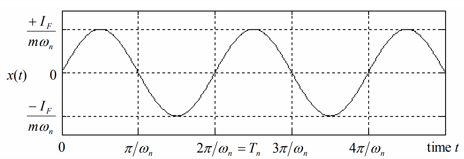
\[x(t)=\omega_{n} \frac{I_{F}}{k} \sin \omega_{n} t=\frac{I_{F}}{m \omega_{n}} \sin \omega_{n} t\label{eqn:8.28} \]

Figure \(\PageIndex{1}\) shows a few cycles of response Equation \(\ref{eqn:8.28}\).

Figure \(\PageIndex{1}\): Ideal impulse response of a mass-spring system