9.1: Homogenous Solutions

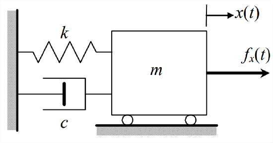
For the mass-dashpot-spring (\(m\)-\(c\)-\(k\)) system of Figure \(\PageIndex{1}\), the equation of motion Equation 3.7.1 derived from Newton’s 2^nd law, with use of the FBD in Figure 3.7.1, is

\[m \ddot{x}+c \dot{x}+k x=f_{x}(t)\label{eqn:9.1} \]

Although 2^nd order systems appear in many different mechanical and electrical forms, the \(m\)-\(c\)-\(k\) system of Figure \(\PageIndex{1}\) is generally considered to be the prototype.

Figure \(\PageIndex{1}\): Mass-dashpot-spring system

To provide direction for developing a standard form of damped 2^nd order ODE, let us consider the homogeneous form of Equation \(\ref{eqn:9.1}\) and seek a homogeneous solution \(x_{h}(t)\) using the conventional method that is described in Section 1.5 [Equation 1.5.3 and the subsequent discussion]:

\[m \ddot{x}_{h}+c \dot{x}_{h}+k x_{h}=0\label{eqn:9.2} \]

We seek \(x_{h}(t)=C e^{\lambda t}\), in which \(C\) and \(\lambda\) are unknown:

\[\Rightarrow\left(m \lambda^{2}+c \lambda+k\right) C e^{\lambda t}=0 \nonumber \]

Now \(x_{h}(t)=C e^{\lambda t} \neq 0\) for a non-trivial solution, leading to the characteristic equation:

\[m \lambda^{2}+c \lambda+k=0\label{eqn:9.3} \]

We solve Equation \(\ref{eqn:9.3}\) for characteristic values \(\lambda\) using the quadratic formula, recognizing \(k / m=\omega_{n}^{2}\) from Equation 7.1.3:

\[\lambda=\frac{-c \pm \sqrt{c^{2}-4 m k}}{2 m}=-\frac{c}{2 m} \pm \sqrt{\left(\frac{c}{2 m}\right)^{2}-\frac{k}{m}}=-\frac{c}{2 m} \pm \sqrt{\left(\frac{c}{2 m}\right)^{2}-\omega_{n}^{2}} \nonumber \]

The dimensionless viscous damping ratio \(\zeta\) and the critical viscous damping constant \(c_c\) are defined as follows:

\[\zeta \equiv \frac{c}{2 m \omega_{n}}=\frac{c}{2 \sqrt{m k}} \equiv \frac{c}{c_{c}} \quad \text { where } \quad c_{c} \equiv 2 m \omega_{n}=2 \sqrt{m k}\label{eqn:9.4} \]

Recall that constants \(m\), \(c\), and \(k\) are normally positive for a passive, stable system, so that \(\zeta\) and \(c_c\) also are normally positive. With definitions Equation \(\ref{eqn:9.4}\), the characteristic values take the form

\[\lambda=-\left(\frac{c}{2 m \omega_{n}}\right) \omega_{n} \pm \sqrt{\left(\frac{c}{2 m \omega_{n}}\right)^{2} \omega_{n}^{2}-\omega_{n}^{2}}=-\zeta \omega_{n} \pm \omega_{n} \sqrt{\zeta^{2}-1}\label{eqn:9.5} \]

Depending upon the value of \(\zeta\) relative to 1, there are three possible distinct solution types for characteristic value \(\lambda\) and the associated homogeneous solution \(x_{h}(t)\):

1. Both roots are real and negative:\[\lambda_{I, I I}=-\zeta \omega_{n} \pm \omega_{n} \sqrt{\zeta^{2}-1}\label{eqn:9.6} \]The corresponding homogeneous solution is an exponentially decaying response with two distinct time constants:\[x_{h}(t)=C_{I} e^{\lambda_{l} t}+C_{I I} e^{\lambda_{I I} t}=C_{I} e^{-t / \tau_{I}}+C_{I I} e^{-t / \tau_{I I}} \quad \text { where } \quad \tau_{I, I I} \equiv-1 / \lambda_{I, I I}\label{eqn:9.7} \]If we were given initial conditions \(x_{h}(0)\) and \(\dot{x}_{h}(0)\), we could now solve for constants and in terms of the ICs, and thus obtain an IC solution for the overdamped \(m\)-\(c\)-\(k\) system. We will obtain such a solution in Section 9.10, using different methods.
2. The two roots Equation \(\ref{eqn:9.5}\) are equal and negative:\[\lambda_{I, I I}=-\omega_{n}\label{eqn:9.8} \]Due to the existence of repeated roots, the homogeneous solution involves both a pure exponential decay term and a term multiplied by time \(t\) that also decays, but more slowly than exponential:\[x_{h}(t)=C_{I} e^{-\omega_{n} t}+C_{I I} t e^{-\omega_{n} t}\label{eqn:9.9} \]The case of critical damping is more of academic than practical interest, since it is rare in practice that physical parameters lead to the exact value \(\zeta=1\). (see homework Problem 9.11)
3. In this case, the terms in Equation \(\ref{eqn:9.5}\) within the square root are negative, so we have two complex characteristic values, each with a negative real part:\[\lambda_{I, I I}=-\zeta \omega_{n} \pm j \omega_{n} \sqrt{1-\zeta^{2}} \equiv-\zeta \omega_{n} \pm j \omega_{d} \quad \text { where } \quad \omega_{d} \equiv \omega_{n} \sqrt{1-\zeta^{2}}\label{eqn:9.10} \]Frequency \(\omega_{d}\) is called the damped natural frequency. The corresponding homogeneous solution is \[x_{h}(t)=C_{I} e^{\lambda_{l} t}+C_{I l} e^{\lambda_{l l} t}=C_{l} e^{\left(-\zeta \omega_{n}+j \omega_{d}\right) t}+C_{I l} e^{\left(-\zeta \omega_{n}-j \omega_{d}\right) t}=e^{-\zeta \omega_{n} t}\left(C_{I} e^{j \omega_{d} t}+C_{I l} e^{-j \omega_{d} t}\right) \nonumber \]By applying Euler’s Equation 2.1.12 and combining constants and appropriately to form two new constants \(D_{I}\) and \(D_{II}\), we can re-write this homogeneous solution in the form of an exponentially decaying sinusoid:\[x_{h}(t)=e^{-\zeta \omega_{n} t}\left(D_{I} \cos \omega_{d} t+D_{I I} \sin \omega_{d} t\right)\label{eqn:9.11} \]If we were given initial conditions \(x_{h}(0)\) and \(\dot{x}_{h}(0)\), we could now solve for real constants \(D_{I}\) and \(D_{II}\) in terms of the ICs, and thus obtain an IC solution for the underdamped \(m\)-\(c\)-\(k\) system. We will obtain this solution in Section 9.4, using the general solution for \(x(t)\) obtained from Laplace transformation. Underdamped systems are the most important and common in practical applications and the most interesting, so we will devote more attention to them than to the other two types of damped 2^nd order systems.