9.2: Standard Form ODE

Last updated
Save as PDF

Page ID: 7678

\( \newcommand{\vecs}[1]{\overset { \scriptstyle \rightharpoonup} {\mathbf{#1}} } \) \( \newcommand{\vecd}[1]{\overset{-\!-\!\rightharpoonup}{\vphantom{a}\smash {#1}}} \)\(\newcommand{\id}{\mathrm{id}}\) \( \newcommand{\Span}{\mathrm{span}}\) \( \newcommand{\kernel}{\mathrm{null}\,}\) \( \newcommand{\range}{\mathrm{range}\,}\) \( \newcommand{\RealPart}{\mathrm{Re}}\) \( \newcommand{\ImaginaryPart}{\mathrm{Im}}\) \( \newcommand{\Argument}{\mathrm{Arg}}\) \( \newcommand{\norm}[1]{\| #1 \|}\) \( \newcommand{\inner}[2]{\langle #1, #2 \rangle}\) \( \newcommand{\Span}{\mathrm{span}}\) \(\newcommand{\id}{\mathrm{id}}\) \( \newcommand{\Span}{\mathrm{span}}\) \( \newcommand{\kernel}{\mathrm{null}\,}\) \( \newcommand{\range}{\mathrm{range}\,}\) \( \newcommand{\RealPart}{\mathrm{Re}}\) \( \newcommand{\ImaginaryPart}{\mathrm{Im}}\) \( \newcommand{\Argument}{\mathrm{Arg}}\) \( \newcommand{\norm}[1]{\| #1 \|}\) \( \newcommand{\inner}[2]{\langle #1, #2 \rangle}\) \( \newcommand{\Span}{\mathrm{span}}\)\(\newcommand{\AA}{\unicode[.8,0]{x212B}}\)

Using the concepts and notation developed in the previous section, we now derive the “standard” form of ODE governing response of damped 2^nd order systems, beginning with ODE Equation 9.1.1 for an \(m\)-\(c\)-\(k\) system:

\[m \ddot{x}+c \dot{x}+k x=f_{x}(t) \Rightarrow \ddot{x}+2 \frac{c}{2 \sqrt{m k}} \sqrt{\frac{k}{m}} \dot{x}+\frac{k}{m} x=\frac{1}{m} f_{x}(t)=\frac{k}{m} \frac{f_{x}(t)}{k}\label{eqn:9.12} \]

Using the definitions from the previous section and the standard input quantity Equation 7.1.4, \(u(t) \equiv f_{x}(t) / k\), we re-write Equation \(\ref{eqn:9.12}\) in the standard form:

\[\ddot{x}+2 \zeta \omega_{n} \dot{x}+\omega_{n}^{2} x=\omega_{n}^{2} u(t)\label{eqn:9.13} \]

In Equation \(\ref{eqn:9.13}\), \(x(t)\) represents any appropriate output quantity (not necessarily just position as in Figure 9.1.1 for a damped 2^nd order system. Recall from Chapter 7 that we can identify \(u(t)\) as being the pseudo-static output, \(x_{p s}(t)\); if \(x(t)\) varies slowly enough that the terms \(\ddot{x}\) and \(2 \zeta \omega_{n} \dot{x}\) are negligible in comparison with \(\omega_{n}^{2} x\), then ODE Equation \(\ref{eqn:9.13}\) reduces to a simple algebraic equation, \(\omega_{n}^{2} x \approx \omega_{n}^{2} u(t)\), the solution of which is the pseudo-static response, \(x(t)=u(t) \equiv x_{p s}(t)\).

Example \(\PageIndex{1}\): the \(LRC\) circuit, a 2^nd order electrical system

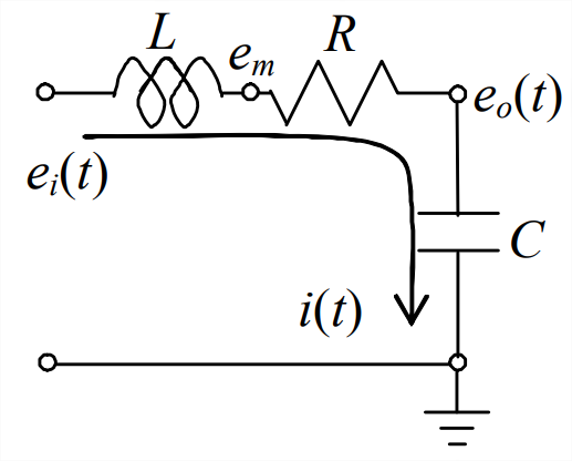
Let us derive an ODE governing the dynamic behavior of the \(LRC\) circuit in the figure below. To write Kirchhoff’s voltage law for this circuit, we start at the input voltage generator and proceed clockwise [see Equation 5.2.10]:

\[\left(e_{i}-0\right)+\left(e_{m}-e_{i}\right)+\left(e_{o}-e_{m}\right)+\left(0-e_{o}\right)=0 \nonumber \]

Next, we substitute in Equation 5.2.9 for the inductor and Ohm’s law Equation 5.2.1 for the resistor:

\[e_{i}+\left(-L \frac{d i}{d t}\right)+(-R i)-e_{o}=0 \Rightarrow L \frac{d i}{d t}+R i+e_{o}=e_{i}(t) \nonumber \]

For the capacitor, we use Equation 5.2.6, then differentiate the result and substitute into the ODE:

\[i=C \frac{d\left(e_{o}-0\right)}{d t}=C \dot{e}_{o} \Rightarrow \frac{d i}{d t}=C \ddot{e}_{o} \Rightarrow L C \ddot{e}_{o}+R C \dot{e}_{o}+e_{o}=e_{i}(t) \nonumber \]

Therefore, we can write the ODE in the standard 2^nd order form Equation \(\ref{eqn:9.13}\) as¹

\[\ddot{e}_{o}+\frac{R}{L} \dot{e}_{o}+\frac{1}{L C} e_{o}=\frac{1}{L C} e_{i}(t) \nonumber \]

From this standard form, we see that the undamped natural frequency is \(\omega_{n}=1 / \sqrt{L C}\), and the viscous damping ratio is \(\zeta=\left(1 / 2 \omega_{n}\right)(R / L)=\frac{1}{2} R \sqrt{C / L}\).

Example \(\PageIndex{2}\): the rate gyroscope, a 2^nd order mechanical system

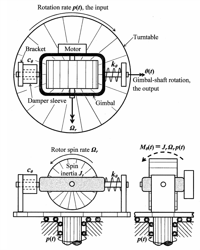
The schematic three-view engineering sketch on the next page represents the basic functional form of a single-axis rate gyroscope (gyro), a sensor of rotational velocity². The supporting turntable in the sketch could be a fixture in a laboratory setup for calibrating the sensor; the turntable rotates clockwise (as viewed from above) with rotational velocity (rate) \(p(t)\). At the heart of the rate gyro is a spinning rotor with polar rotational inertia \(J_r\) about its spin axis; it is driven by a motor to spin counterclockwise (as viewed from the front) at the high constant spin rate (rotational speed) \(\Omega_{r}\), which is usually orders of magnitude greater than \(|p(t)|\). The motor and spinning rotor are attached to a gimbal (rotating frame) and shaft segments that fit into bearings within brackets projecting from the turntable. The gimbal-shaft assembly (including the motor and spinning rotor) can rotate through small angle \(\theta(t)\) about the so-called “gimbal axis”. This \(\theta(t)\) rotation is resisted by a rotational spring with constant \(k_{\theta}\), and by a rotational viscous damper with constant \(c_{\theta}\). (Drag is imposed by viscous liquid within a gap between the outer surface of the shaft segment and the inner surface of the sleeve, which is attached to the bracket.) The polar rotational inertia of the gimbal-shaft assembly about the gimbal axis is \(J_{\theta}\). Due to the inertia \(J_{r}\) and high speed \(\Omega_{r}\) of the spinning rotor, turntable rotation \(p(t)\) induces an inertial moment about the gimbal axis, \(M_{\theta}(t)=J_{r} \Omega_{r} p(t) \cos \theta(t)\) [as derived from Newton’s laws of rigid-body dynamics by, e.g., Cannon, 1967, pages 152-163]; we assume that \(\theta(t)\) is small enough that \(\cos \theta(t) \approx 1\), so that \(M_{\theta}(t) \approx J_{r} \Omega_{r} p(t)\), as labeled on the sketch. From Equation 3.3.2, Newton’s 2^nd law for rotation of the gimbal-shaft assembly about the gimbal axis is

\[\Sigma(\text { Moments })_{\text {about } ~ g i m b a l ~ a x i s ~}=(\text { rotational inertia) } \times(\text { rotational acceleration) })_{\text{about gimbal axis}} \nonumber \]

\[M_{\theta}(t)-c_{\theta} \dot{\theta}-k_{\theta} \theta=J_{\theta} \ddot{\theta} \quad \Rightarrow \quad J_{\theta} \ddot{\theta}+c_{\theta} \dot{\theta}+k_{\theta} \theta=J_{r} \Omega_{r} p(t) \nonumber \]

Therefore, we can write the ODE in the standard 2^nd order form Equation \(\ref{eqn:9.13}\) as

\[\ddot{\theta}+\frac{c_{\theta}}{J_{\theta}} \dot{\theta}+\frac{k_{\theta}}{J_{\theta}} \theta=\frac{J_{r} \Omega_{r}}{J_{\theta}} p(t)=\frac{k_{\theta}}{J_{\theta}} \frac{J_{r} \Omega_{r}}{k_{\theta}} p(t) \nonumber \]

From this standard form, we see that the undamped natural frequency is \(\omega_{n}=\sqrt{k_{\theta} / J_{\theta}}\), and the viscous damping ratio is \(\zeta=\left(c_{\theta} / J_{\theta}\right) /\left(2 \omega_{n}\right)\), and the standard input quantity, with the same dimensions as rotation-angle output \(\theta(t)\), is \(u(t)=\left(J_{r} \Omega_{r} / k_{\theta}\right) p(t) \equiv \theta_{p s}(t)\), the pseudo-static output.

In practical application of a rate gyro, a transducer detects the rotation of the gimbal-shaft assembly and generates an electrical signal proportional to \(\theta(t)\), which might be displayed and/or recorded by a data-acquisition-and-processing system, and might also serve as an input to a control system. Spinning-rotor rate gyros come in various sizes and shapes; typical units are around the size of a one- or two-pound can of vegetables, and their cases can be cylindrical or box-shaped³.

¹In Appendix B, Section 19.3, this ODE is derived by an alternative method using energy and power. The rate of change of system energy is equated with the power supplied to the system.

²Gyroscopes have been used in sensors and actuators for both aerospace vehicles and water-borne vehicles. Some examples are described by Cannon, 1967, pages 159-163, 617-626, 696-697, and by Den Hartog, 1956, pages 108-112.

³This type of spinning-rotor gyro can be considered a “legacy” design, not necessarily the most modern or the best for current applications. Rotation sensors using laser optics and microelectromechanics (MEMS) have been developed more recently.