11.1: Equations of Motion for a Rigid Body in General Plane Motion

Consider a rigid body that is restricted to motion in the \(xy\) plane. Figure \(\PageIndex{1}\) shows the body in its reference static equilibrium position (solid lines) and in a position of motion (dashed lines) relative to the reference position. The \(xy\) axis system shown is an inertial reference with its origin at point \(O\), which is either motionless or translating at a constant velocity. We will use vectors and vector operations, so we need to recognize that the inertial reference system is really the three-dimensional Cartesian \(xyz\) axis system, with the \(z\) axis being perpendicular to the \(xy\) plane and pointed toward us, in the sense of the right-hand rule. We denote the fixed unit vectors in the reference Cartesian directions as \(\mathbf{1}_{\mathbf{x}}\), \(\mathbf{1}_{\mathbf{y}}\), and \(\mathbf{1}_{\mathbf{z}}\). From the background of your previous dynamics and physics courses, you should be familiar with vectors, vector algebra and calculus, and vector kinematics and dynamics; if necessary, you should review these concepts in your engineering dynamics textbook.

Figure \(\PageIndex{1}\): Rigid body in general plane motion

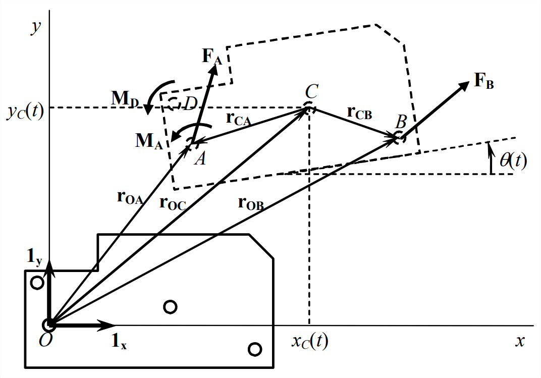
Of particular interest is the position and orientation of the rigid body’s center of mass \(C\). At any instant of time \(t\), \(C\) has relative position coordinates \(\left[x_{C}(t), y_{C}(t)\right]\). Thus, the vector position of \(C\) relative to some absolutely fixed point \(P\) is \(\mathbf{r}_{\mathbf{C}}(t)=\mathbf{r}_{\mathbf{o}}(t)+\mathbf{r}_{\mathbf{o C}}(t)=\mathbf{r}_{\mathbf{o}}(t)+x_{C}(t) \mathbf{1}_{\mathbf{x}}+y_{C}(t) \mathbf{1}_{\mathbf{y}}\), where is the known instantaneous position of \(O\) relative to \(P\). Similarly, the vector velocity of \(C\) relative to absolutely fixed point \(P\) is \(\mathbf{v}_{\mathbf{C}}(t)=\mathbf{v}_{\mathbf{o}}(t)+\mathbf{v}_{\mathbf{O C}}(t)=\mathbf{v}_{\mathbf{o}}(t)+\dot{x}_{C}(t) \mathbf{1}_{\mathbf{x}}+\dot{y}_{C}(t) \mathbf{1}_{\mathbf{y}}\), where \(\mathbf{v}_{\mathbf{o}}(t)\) is the constant velocity of \(O\) relative to \(P\). Because \(\mathbf{v}_{\mathbf{o}}(t)\) is constant, the absolute vector acceleration of \(C\) is \(\mathbf{a}_{\mathrm{C}}(t)=\mathbf{a}_{\mathrm{oc}}(t)=\ddot{x}_{C}(t) \mathbf{1}_{\mathrm{x}}+\ddot{y}_{C}(t) \mathbf{1}_{\mathrm{y}}\). We denote as \(\theta(t)\) the positive-counterclockwise rotational orientation of mass center \(C\) (indeed, of the entire body, since it is rigid). Position \(\mathbf{r}_{\mathbf{O}}(t)\) of \(O\) is known, so if we can determine at any instant the three motion quantities \(x_{C}(t)\), \(y_{C}(t)\), and \(\theta(t)\), then we can calculate from simple geometry the position of any point on the rigid body. These three quantities are independent in general plane motion, and only these three [plus known \(\mathbf{r}_{\mathbf{O}}(t)\)] are required to describe completely the position in space of the rigid body. Therefore, \(x_{C}(t)\), \(y_{C}(t)\), and \(\theta(t)\) are called degrees of freedom, and general plane rigid-body motion is called a three-degrees-of-freedom (3-DOF) problem.

For generality, we identify three other points fixed to the rigid body, at which point actions (forces or moments) are applied by sources external to the body. (In general, there can be more or fewer points of externally applied actions; analyzing such situations will require only minor modifications to the present derivation.) Point \(A\) is a connection to the external environment, possibly through springs, dampers, etc.; actions applied at Point A are vector reaction force \(\mathbf{F}_{\mathrm{A}}=F_{A x} \mathbf{1}_{\mathbf{x}}+F_{A y} \mathbf{1}_{\mathbf{y}}\) and vector reaction moment \(\mathbf{M}_{\mathrm{A}}=M_{A} \mathbf{1}_{\mathbf{z}}\). It is useful to express the vector position of point A in terms of that of mass center \(C\): \(\mathbf{r}_{\mathbf{O A}}=\mathbf{r}_{\mathbf{O C}}+\mathbf{r}_{\mathbf{C A}}\) (see Figure \(\PageIndex{1}\)). An arbitrary vector force \(\mathbf{F}_{\mathbf{B}}=F_{B x} \mathbf{1}_{\mathbf{x}}+F_{B y} \mathbf{1}_{\mathbf{y}}\) is applied at point \(B\), and that point’s vector position is expressed as \(\mathbf{r}_{\mathrm{OB}}=\mathbf{r}_{\mathrm{OC}}+\mathbf{r}_{\mathrm{CB}}\). Finally, an arbitrary vector moment \(\mathbf{M}_{\mathbf{D}}=M_{D} \mathbf{1}_{\mathbf{z}}\) acts at point \(D\).

We denote as \(m\) the mass of the rigid body. Newton’s 2^nd law for forces, written in vector form, is

\[m \mathbf{a}_{\mathrm{C}}=\mathbf{F}_{\mathrm{A}}+\mathbf{F}_{\mathrm{B}}\label{eqn:11.1} \]

Expressing Equation \(\ref{eqn:11.1}\) in terms of scalar components gives the two scalar ODEs:

\[m \ddot{x}_{C}=F_{A x}+F_{B x}\label{eqn:11.2a} \]

\[m \ddot{y}_{C}=F_{A y}+F_{B y}\label{eqn:11.2b} \]

We denote as \(J_C\) the rotational inertia of the rigid body about an axis normal to the plane of motion and passing through mass center \(C\). Newton’s 2^nd law for moments relevant to this plane-motion case states that the inertial moment about mass center \(C\) equals the sum of all applied moments about mass center \(C\); it is expressed as follows in vector notation, including vector cross products:

\[J_{C} \ddot{\theta} \mathbf{1}_{\mathbf{z}}=\mathbf{r}_{\mathrm{CA}} \times \mathbf{F}_{\mathbf{A}}+\mathbf{r}_{\mathrm{CB}} \times \mathbf{F}_{\mathbf{B}}+\left(M_{A}+M_{D}\right) \mathbf{1}_{\mathbf{z}}\label{eqn:11.3} \]

Despite the vector notation, Equation \(\ref{eqn:11.3}\) is actually a scalar equation, because the vector cross products obviously produce vectors in the \(z\) direction; the use of these cross products just provides economy of notation¹.

We shall see an application of general-plane-motion Equations \(\ref{eqn:11.2a}\), \(\ref{eqn:11.2b}\), and \(\ref{eqn:11.3}\) to a specific aeroelastic system in Section 11.3 (Example 11-3); but, first, it is appropriate to develop in Section 11.2 and to illustrate in Section 11.3 (Examples 11-1 and 11-2) the special case of pure plane rotational motion about a fixed point.

¹For Equations \(\ref{eqn:11.2a}\), \(\ref{eqn:11.2b}\), and \(\ref{eqn:11.3}\), the reference \(xyz\) axis system is inertial, either stationary in space or moving at a constant translational velocity, and motion of the rigid body is measured relative to this inertial system. However, for many problems in dynamics, it is preferable to derive equations of motion using a reference axis system that is fixed in the body and moves with it. A plane-motion problem of this type is the leadinglagging rotation of a hinged helicopter rotor blade, as analyzed by Bramwell, 1976, pp. 51-52.