11.3: Examples

Example \(\PageIndex{1}\): damped, spring-supported rigid bar, hinged at point \(H\)

Let us derive the specific ODE of motion for the system of Figure \(\PageIndex{1}\), assuming small angles of rotation. The bar has rotational inertia \(J_{H}\) about hinge \(H\), which we assume to have negligible friction. The bar is shown in the reference static equilibrium position, subject to static gravity but before applied dynamic force \(F(t)\) becomes active. Dynamic degree of freedom \(\theta(t)\) shown with dashed lines is the small rotation relative to the static equilibrium position. (It is this book’s graphical convention for this and all subsequent systems of this type that the rigid body is drawn in its static equilibrium position, and dynamic motion relative to this reference position is indicated with dashed lines and annotation.) Note the rotation spring with spring constant \(k_{\theta}\) at hinge \(H\); this spring resists rotation by generating an opposing moment of magnitude \(k_{\theta} \times \theta\). Typical units for \(k_{\theta}\) are lb-inch/radian and N-m/radian.

Figure \(\PageIndex{1}\): Example 11.3.1: damped, spring-supported, hinged rigid bar

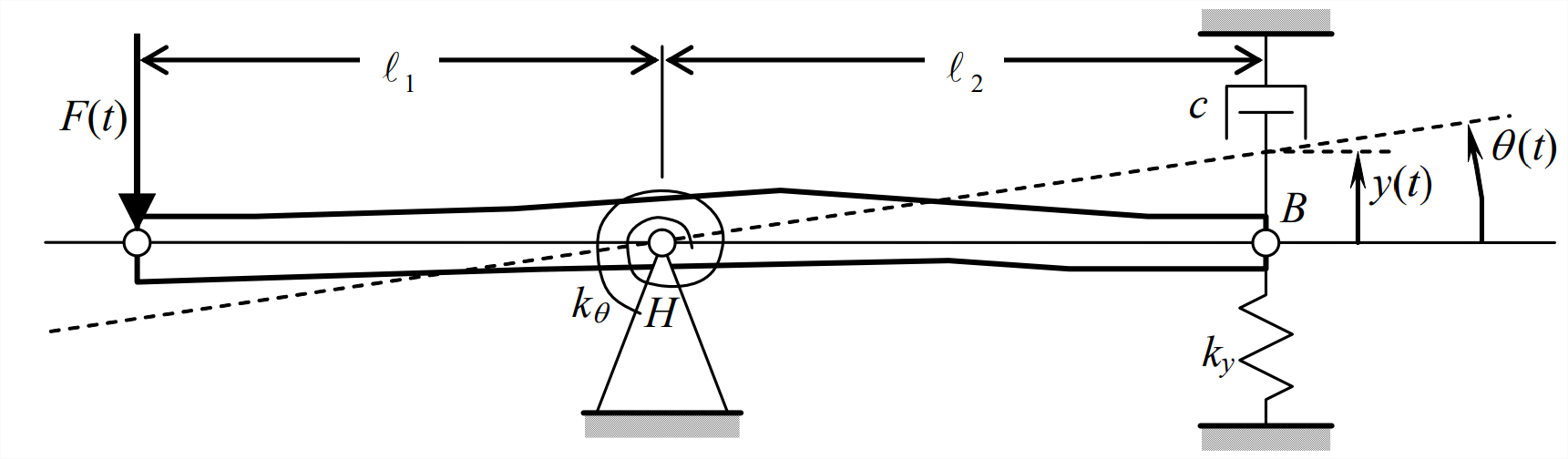
Before drawing a dynamic free-body diagram (DFBD, as defined in Section 7.5), we need to express appropriately the reaction forces on the bar at point \(B\) from the translational spring (\(k_{y} \times y\)) and the translational viscous damper (\(c \times \dot{y}\)). Observe that point \(B\) moves in a circular arc of radius \(\ell_{2}\), so that \(y=\ell_{2} \sin \theta\). For arbitrarily large \(\theta\), the term \(\sin \theta\) and its time derivative would make equation of motion Equation 11.2.10 nonlinear. However, the assumption of small rotation, \(|\theta(t)|<\approx 10^{\circ}\), linearizes that ODE; the geometry of small rotation gives approximate linear equations in terms of \(\theta\) for stretch \(y\) of the translational spring due to motion of point \(B\), and for damper-piston velocity \(\dot{y}\):

\[y=\ell_{2} \sin \theta \approx \ell_{2} \theta(\theta \text { in radians }), \quad \text { and } \quad \dot{y}=\ell_{2} \cos \theta \times \dot{\theta} \approx \ell_{2} \dot{\theta} \nonumber \]

The geometry of small rotation was used previously in the example of Section 7.1 to linearize the pendulum equation of motion. For the system of Figure \(\PageIndex{1}\), the assumption of small rotation is physically plausible as well as mathematically expedient, because the translational and rotational springs most likely would restrict rotation of the bar to small angles relative to the static equilibrium position.

The appropriate DFBD is drawn below. Note that we do not include bar weight among the applied forces. We omit bar weight because we are interested only in dynamic motion relative to the static equilibrium position, and because this bar is approximately horizontal so that gravity has no pendulous effect on it; if you are not sure why we neglect weight in this case, then review Section 7.5.

Figure \(\PageIndex{2}\)

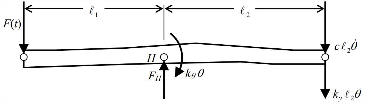
From the DFBD and Equation 11.2.10, the ordinary differential equation of motion is

\[J_{H} \ddot{\theta}=\ell_{1} F(t)-k_{\theta} \theta-\ell_{2}\left(c \ell_{2} \dot{\theta}+k_{y} \ell_{2} \theta\right) \nonumber \]

\[\Rightarrow \quad J_{H} \ddot{\theta}+c \ell_{2}^{2} \dot{\theta}+\left(k_{\theta}+k_{y} \ell_{2}^{2}\right) \theta=\ell_{1} F(t)\label{eqn:11.12} \]

Equation \(\ref{eqn:11.12}\) can be put into the standard form for a 2^nd order damped system, and all of the relevant results of Chapters 9 and 10 can be expressed in terms of the physical parameters of this particular mechanical system. For example, we can immediately find equations for the system undamped natural frequency and viscous damping ratio:

\[\omega_{n}=\sqrt{\frac{k_{\theta}+k_{y} \ell_{2}^{2}}{J_{H}}}, \quad 2 \zeta \omega_{n}=\frac{c \ell_{2}^{2}}{J_{H}} \Rightarrow \zeta=\frac{1}{2} \frac{c \ell_{2}^{2}}{\sqrt{J_{H}\left(k_{\theta}+k_{y} \ell_{2}^{2}\right)}}\label{eqn:11.13} \]

NOTE: It is easy to make mistakes in algebra when we derive results such as Equations \(\ref{eqn:11.13}\). One good, easy type of partial check that you can use is to evaluate the physical dimensions of algebraic results. (It is only a partial check because dimensional consistency is a necessary condition, but it does not guarantee the correctness of an algebraic equation.) Do Equations \(\ref{eqn:11.13}\) have the correct physical dimensions? You should be able to show that the equation for \(\omega_{n}\) has the dimension (time)^-1 and that the equation for \(\zeta\) is dimensionless. Do not forget that rotation \(\theta\) is dimensionless and that the radian, the natural metric of rotation, is unitless. If you are more comfortable working with units than dimensions, it is satisfactory to check units instead. Table 3.1.1 should be helpful relative to mechanical units.

Example \(\PageIndex{2}\): 1-DOF typical-section model for study of aerolastic wing twist

Since the beginning of modern aeronautical engineering in the late 1800s and early 1900s, the interaction of aerodynamic pressure with airplane structural flexibility has often produced unexpected and sometimes disastrous consequences. The subject of these phenomena became known as aeroelasticity. During and after World War I, highaspect-ratio, cantilevered monoplane wings tended to be susceptible both to aeroelastic flutter, undamped vibration that can escalate to destruction of wing and airplane, and to aeroelastic divergence, the gradual twisting-off of a wing in, for example, pull-up from a dive¹. In their attempts to analyze these aeroelastic phenomena, early aeronautical engineers used simplified, low-degrees-of-freedom dynamic models of wing structures. The basis of these models is called a typical section: one “typical” cross-section of a high-aspect-ratio, straight, unswept wing is treated aerodynamically as an airfoil in twodimensional flow (without spanwise flow), and structurally as a spring-supported rigid body (without spanwise beam bending and twisting).

The simplest typical-section model is the one-degree-of-freedom (1-DOF) system drawn in Figure \(\PageIndex{3}\). It is helpful to visualize this as a physical model mounted for testing in a wind tunnel. Elastic axis EA (the hinge) is assumed to be frictionless, and rotation spring \(k_{\theta}\) represents wing torsional stiffness. (The term elastic axis refers to the line along the span of a high-aspect-ratio, straight, unswept wing about which the wing chordwise sections rotate if a pure twisting moment is imposed upon the wing.) This model is intended primarily for the study of aeroelastic divergence. Figure \(\PageIndex{3}\) shows the typical

Figure \(\PageIndex{3}\): Example 11.3.2: 1-DOF typical section in an airstream

section in the reference static equilibrium position before the wind tunnel fan is turned on. Turning on the wind tunnel fan then produces an airstream of steady free-stream velocity \(V\) flowing over the typical section at small angle of incidence \(\alpha_{r}\) relative to the reference chordline of the typical section. The airstream creates a resultant lifting force \(F_L\) that acts through aerodynamic center \(AC\), and a resultant pitching moment \(M_{AC}\) that acts about \(AC\). For most cases of practical interest, \(AC\) is forward of \(EA\) by some positive distance \(e\), as shown on Figure \(\PageIndex{3}\); the polarity \(e > 0\) is very important relative to divergence. Aerodynamic actions \(F_L\) and \(M_{AC}\) impose moments upon rotation spring \(k_{\theta}\), and the spring flexibility permits structural rotation \(\theta\) relative to the reference position.

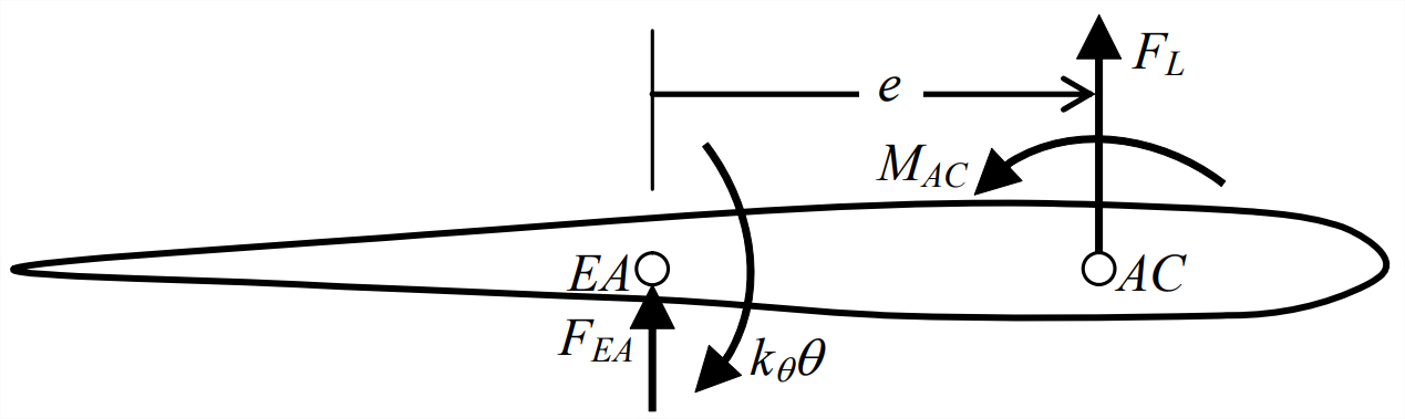
The DFBD associated with Figure \(\PageIndex{3}\) is drawn below. The equation of motion comes directly from the DFBD and Equation 11.2.10, with the assumption of small angles of incidence and rotation, \(\left|\alpha_{r}\right|<\approx 10^{\circ}\) and \(|\theta(t)|<\approx 10^{\circ}\), and with \(J_{E A}\) being the rotational inertia of the typical section about \(EA\):

\[J_{E A} \ddot{\theta}=F_{L} e+M_{A C}-k_{\theta} \theta \Rightarrow J_{E A} \ddot{\theta}+k_{\theta} \theta=F_{L} e+M_{A C}\label{eqn:11.14} \]

Figure \(\PageIndex{4}\)

We can cast Equation \(\ref{eqn:11.14}\) into a more interesting and useful form by relating the aerodynamic actions to the structural rotation. We assume that the airstream direction coincides with the zero-lift attitude of the airfoil, i.e., that \(F_L\) would be zero for any value of airspeed \(V\) if the airfoil incidence were fixed at \(\alpha_{r}=0\). Consequently, the total angle of attack of the airfoil relative to the zero-lift attitude is \(\alpha=\alpha_{r}+\theta\). Then aerodynamic lift and moment can be expressed as

\[F_{L}=\bar{q} S C_{L \alpha} \alpha=\bar{q} S C_{L \alpha}\left(\alpha_{r}+\theta\right), \quad \text { and } \quad M_{A C}=\bar{q} S c C_{M A C}\label{eqn:11.15} \]

Note especially in Equations \(\ref{eqn:11.15}\) that an aerodynamic action (in this case, lift \(F_L\)) is dependent upon structural deformation (in this case, rotation \(\theta\)); this type of interaction between aerodynamics and structural flexibility is an important characteristic of all aeroelastic phenomena. The symbols used in Equations \(\ref{eqn:11.15}\) beyond those previously defined are:

\(\bar{q}=\frac{1}{2} \rho V^{2}\) is the free-stream dynamic pressure (lb/ft² or N/m²).

\(\rho\) is air density (slug/ft³ or kg/m³).

\(S=b c\) is the planform area of the typical section (ft² or m²).

\(b\) is the span of the typical section into the plane of the paper (ft or m).

\(C_{L \alpha}>0\) is the slope of the curve of section lift coefficient (\(F_{L} / \bar{q} S\)) versus angle of attack (rad^-1), which we assume here to be constant for small angles of attack.

\(C_{M A C}\) is the dimensionless coefficient of pitching moment about \(AC\), normally positive for a positively cambered airfoil, but zero for an uncambered thin airfoil.

Wind tunnel experiments and aerodynamic theory show that aerodynamic action Equations \(\ref{eqn:11.15}\) are valid only for steady flow, for which angle of attack \(\alpha\) does not vary with time. However, we will approximate a bit here and assume that Equations \(\ref{eqn:11.15}\) are at least qualitatively valid for slowly-time-varying angle of attack, \(\alpha(t)=\alpha_{r}+\theta(t)\). This approximation is sometimes called quasi-static or quasi-steady aerodynamics. Substituting Equations \(\ref{eqn:11.15}\) into Equation \(\ref{eqn:11.14}\) gives

\[J_{E A} \ddot{\theta}+k_{\theta} \theta=\bar{q} S C_{L \alpha}\left(\alpha_{r}+\theta\right) e+\bar{q} S c C_{M A C} \nonumber \]

\[\Rightarrow \quad J_{E A} \ddot{\theta}+\left(k_{\theta}-\bar{q} S C_{L \alpha} e\right) \theta=\bar{q} S C_{L \alpha} \alpha_{r} e+\bar{q} S c C_{M A C}\label{eqn:11.16} \]

Note in Equation \(\ref{eqn:11.16}\) that the total stiffness constant, \(k_{\theta}-\bar{q} S C_{L \alpha} e\) (structural stiffness plus aerodynamic “stiffness”) can, for \(e > 0\), become zero or even negative if dynamic pressure \(\bar{q}\) is sufficiently large. This is critically important relative to the stability of the system. Consider steady flow, for example, for which \(\ddot{\theta}=0\); in this case we can solve Equation \(\ref{eqn:11.16}\) algebraically for the static structural rotation:

\[\theta=\frac{\bar{q} S\left(C_{L \alpha} \alpha_{r} e+c C_{M A C}\right)}{k_{\theta}-\bar{q} S C_{L \alpha} e} \equiv \frac{\bar{q}\left(C_{L \alpha} \alpha_{r} e+c C_{M A C}\right)}{C_{L \alpha} e\left(\bar{q}_{D}-\bar{q}\right)}\label{eqn:11.17} \]

In Equation \(\ref{eqn:11.17}\), we define the divergence dynamic pressure in terms of other fixed system parameters as

\[\bar{q}_{D} \equiv \frac{k_{\theta}}{S C_{L \alpha} e}\label{eqn:11.18} \]

If it is possible for a given set of physical parameters to increase the wind-tunnel airspeed \(V\) up to the point that \(\bar{q} \rightarrow \bar{q}_{D}=k_{\theta} / S C_{L \alpha} e\), then, from Equation \(\ref{eqn:11.17}\), clearly something very interesting will happen. From your knowledge of aerodynamics and structures, what types of physical behavior do you think are possible? Keep in mind that Equation \(\ref{eqn:11.17}\) is predicated on the assumptions of small angles and complete linearity of both aerodynamics and structures (in this system, the rotation spring).

A conventional airplane control surface is mounted on the trailing edge of a major lifting surface, with the leading edge of the control surface hinged to the lifting surface (e.g., an aileron on a wing). In this case, the aerodynamic center of the control surface is aft of the elastic axis, making the moment arm \(e\) negative (see Figure \(\PageIndex{3}\)). From Equation \(\ref{eqn:11.17}\), this produces the negative moment \(\bar{q} S C_{L \alpha} \alpha_{r} e\), which is called a blowdown moment, and it also augments the structural stiffness in the total stiffness constant \(k_{\theta}-\bar{q} S C_{L \alpha} e\). Therefore, a conventional trailing-edge control surface cannot diverge aeroelastically.

Example \(\PageIndex{3}\): 2-DOF typical-section model for coupled wing being and torsion

We now return to general-plane-motion Equations 11.1.2, 11.1.3, and 11.1.4, which are three ODEs in three unknown DOFs: \(x_{C}(t)\), \(y_{C}(t)\), and \(\theta(t)\). In practice, these ODEs are often coupled by system geometry and the nature of the active and reactive actions. Moreover, if motion is allowed to have arbitrarily large magnitude, then the equations are usually nonlinear. In general, these arbitrary-plane-motion equations can be solved only in numerical form, not in the form of algebraic equations. However, the mechanical systems considered in this book are limited, in most cases, to those for which center-of-mass translation is small relative to rigid-body dimensions, and for which rotation is small, \(|\theta(t)|<\approx 10^{\circ}\) (e.g., Examples 11.3.1 and 11.3.2 in this section); these limitations allow us to linearize the ODEs into more easily solvable forms.

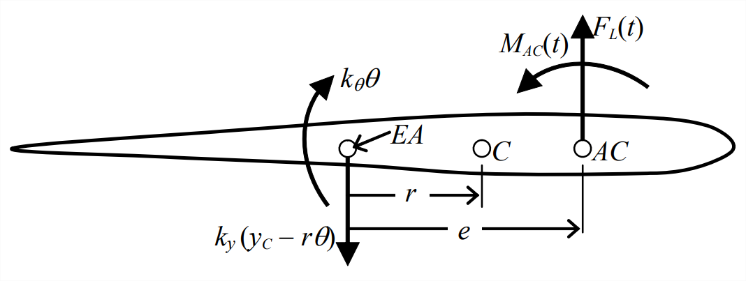
One of the first forms of aeroelastic wing flutter that was observed and carefully analyzed during the early 1900s involves coupled bending and torsional vibration (Bisplinghoff et al., 1955, Section 9.2). The two-degrees-of-freedom (2-DOF) typical section depicted in Figure \(\PageIndex{5}\) is a very simplified structural model used to study wing bending-torsion flutter². The airfoil section is hinged without friction at elastic axis \(EA\) to a vertical bar (assumed rigid and of negligible inertial force), which is restricted to vertical translation by frictionless linear bearings. Rotational spring \(k_{\theta}\) simulates wing torsional stiffness, and translational spring \(k_{y}\) simulates wing bending stiffness. The theory of unsteady aerodynamics, even for two-dimensional flow, is very complicated, so we shall simply represent the aerodynamic resultant actions generally as lift \(F_{L}(t)\) and pitching moment about the aerodynamic center \(M_{A C}(t)\), and we shall focus on the structural dynamics.

Figure \(\PageIndex{5}\): Example 11.3.3: 2-DOF typical section

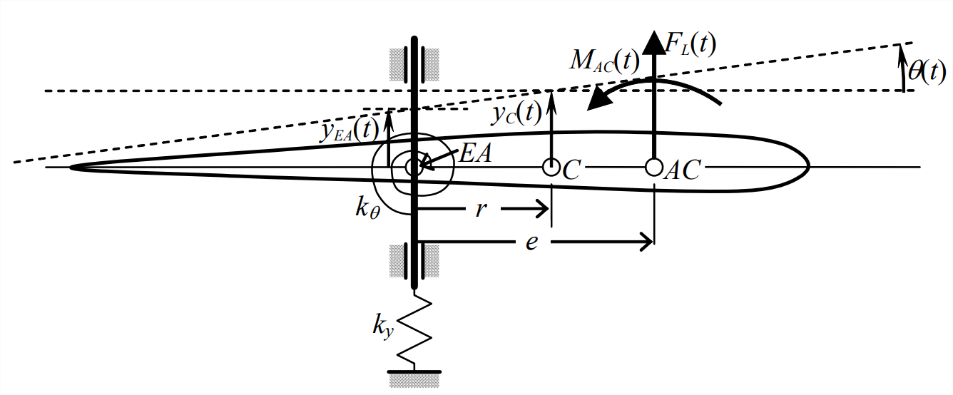
In order to write the equations of motion for this typical section, we select as degrees of freedom the vertical translation \(y_C(t)\) of mass center \(C\), and pitching rotation \(\theta(t)\), both relative to the reference static equilibrium position. The geometry of small rotation is represented by the relationship between \(y_{\mathrm{C}}(t)\) and \(y_{E A}(t)\):

\[y_{C}(t)=y_{E A}(t)+r \sin \theta(t) \approx y_{E A}(t)+r \theta(t) \Rightarrow y_{E A}(t) \approx y_{C}(t)-r \theta(t)\label{eqn:11.19} \]

The DFBD associated with Figure \(\PageIndex{5}\) is drawn below, with approximation Equation \(\ref{eqn:11.19}\) used to annotate the force due to translation spring \(k_{y}\).

Figure \(\PageIndex{6}\)

Using this DFBD, we write the two relevant equations of motion, Equations 11.1.3 and 11.1.4 in scalar form, as

\[m \ddot{y}_{C}=F_{L}(t)-k_{y}\left(y_{C}-r \theta\right)\label{eqn:11.20a} \]

\[J_{C} \ddot{\theta}=(e-r) F_{L}(t)+M_{A C}(t)-k_{\theta} \theta+r k_{y}\left(y_{C}-r \theta\right)\label{eqn:11.20b} \]

It is appropriate to express Equations \(\ref{eqn:11.20a}\) \(\ref{eqn:11.20b}\) with all terms involving degrees of freedom \(y_{C}(t)\) and \(\theta(t)\) transposed to the left-hand sides:

\[m \ddot{y}_{C}+k_{y} y_{C}-r k_{y} \theta=F_{L}(t)\label{eqn:11.21a} \]

\[J_{C} \ddot{\theta}-r k_{y} y_{C}+\left(k_{\theta}+r^{2} k_{y}\right) \theta=(e-r) F_{L}(t)+M_{A C}(t)\label{eqn:11.21b} \]

Equations \(\ref{eqn:11.21a}\) and \(\ref{eqn:11.21b}\) are a pair of 2^nd order, coupled ODEs in unknowns \(y_{C}(t)\) and \(\theta(t)\). Just as Equations \(\ref{eqn:11.15}\), Equations \(\ref{eqn:11.21a}\) and \(\ref{eqn:11.21b}\) are described as being coupled because each equation contains both dependent variables and neither equation can be solved independently of the other. It is possible, though we will not bother doing it, to combine these two equations into a single 4^th order ODE in a single unknown function of time; therefore, this 2-DOF typical section is actually a 4th order system. It is appropriate and common also to express the set of ODEs Equations \(\ref{eqn:11.21a}\) and \(\ref{eqn:11.21b}\) in matrix form:

\[\overbrace{\left[\begin{array}{cc}
m & 0 \\
0 & J_{C}
\end{array}\right]}^{\text {inertia matrix }}\left[\begin{array}{c}
\ddot{y}_{C} \\
\ddot{\theta}
\end{array}\right] + \overbrace{\left[\begin{array}{cc}
k_{y} & -r k_{y} \\
-r k_{y} & k_{\theta}+r^{2} k_{y}
\end{array}\right]}^{\text{structural stiffness matrix}}\left[\begin{array}{c}
y_{C} \\
\theta
\end{array}\right] = \left[\begin{array}{c}
F_{L}(t) \\
(e-r) F_{L}(t)+M_{A C}(t)
\end{array}\right] \label{eqn:11.22} \]

The labeled left-hand-side coefficient matrices of Equation \(\ref{eqn:11.22}\) are typical for structural dynamic systems, and they exhibit some important general properties. The inertia matrix in this case is diagonal; more generally, it will be non-diagonal but symmetric. The inertia matrix will always be positive definite because all matter has positive mass; therefore, the determinant of the inertia matrix will always be positive. In Equation \(\ref{eqn:11.22}\), that determinant is simply the product \(m J_{C}>0\). The structural stiffness matrix in Equation \(\ref{eqn:11.22}\) is symmetric, and this is a general property resulting from linearity between applied actions and structural deformations. Moreover, if a structure is restrained by grounded supports, such as the rotational spring \(k_{\theta}\) and translational spring \(k_{y}\) of the typical section, then each of the diagonal elements of the stiffness matrix will be positive, and the stiffness matrix itself will be positive definite. You can check easily that the determinant of the stiffness matrix in Equation \(\ref{eqn:11.22}\) is the product \(k_{y} k_{\theta}>0\). The coupling between vertical translation \(y_{C}(t)\) and pitching rotation \(\theta(t)\) of the typical section is both produced by and displayed by the non-zero off-diagonal terms of the stiffness matrix, each being \(-r k_{y}\).

¹For the early history of aeroelastic divergence, see Bisplinghoff et al., 1955, pp. 3-7, and Gordon, 1978, pp. 259-270.

²Physical typical-section airfoils were designed, fabricated, and tested in recent wind-tunnel experimental research studies of unsteady aerodynamics (as summarized by Bennett, 2000), and of feedback control to suppress flutter (DeMarqui, et al., 2005 and 2006). Homework Problem 16.11 applies an approximate theory of unsteady aerodynamics in a simulation of one such experimental project.