12.3: Vibration Modes of an Undamped Typical Model of a Wing

From Example 11.3.3 of Section 11.3, the system is depicted again in Figure \(\PageIndex{1}\):

Figure \(\PageIndex{1}\): 2-DOF typical section

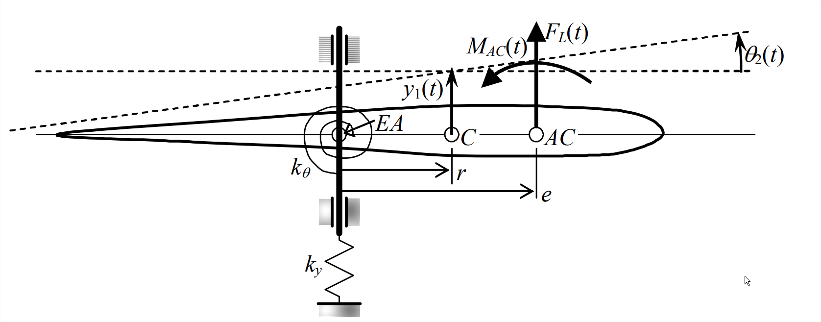
The degree-of-freedom symbols \(y_{C}(t)\) and \(\theta(t)\) used in Chapter 11 are changed here, respectively, to \(y_{1}(t)\) and \(\theta_{2}(t)\), in order to denote clearly that these motion quantities are, respectively, degrees of freedom (DOFs) #1 and #2.

The matrix equation of motion in DOFs \(y_{1}(t)\) and \(\theta_{2}(t)\), from Equation 11.3.16 is

\[\left[\begin{array}{cc}
m & 0 \\
0 & J_{C}
\end{array}\right]\left[\begin{array}{c}
\ddot{y}_{1} \\
\ddot{\theta}_{2}
\end{array}\right]+\left[\begin{array}{cc}
k_{y} & -r k_{y} \\
-r k_{y} & k_{\theta}+r^{2} k_{y}
\end{array}\right]\left[\begin{array}{c}
y_{1} \\
\theta_{2}
\end{array}\right]=\left[\begin{array}{c}
F_{L}(t) \\
(e-r) F_{L}(t)+M_{A C}(t)
\end{array}\right]\label{eqn:12.25} \]

To analyze Equation \(\ref{eqn:12.25}\) for modes of free vibration following the procedure described in the previous section, we set to zero the applied aerodynamic actions, and we seek motion solutions of the unforced system in the form:

\[\left[\begin{array}{l}
y_{1}(t) \\
\theta_{2}(t)
\end{array}\right]=\left[\begin{array}{l}
Y_{1} \\
\Theta_{2}
\end{array}\right] \cos \omega t\label{eqn:12.26} \]

Substituting Equation \(\ref{eqn:12.26}\) into Equation \(\ref{eqn:12.25}\), canceling the common \(\cos \omega t\) term, and collecting all coefficients in a single square matrix leads to

\[\left[\begin{array}{cc}
k_{y}-\omega^{2} m & -r k_{y} \\
-r k_{y} & k_{\theta}+r^{2} k_{y}-\omega^{2} J_{C}
\end{array}\right]\left[\begin{array}{c}
Y_{1} \\
\Theta_{2}
\end{array}\right]=\left[\begin{array}{l}
0 \\
0
\end{array}\right]\label{eqn:12.27} \]

Setting to zero the determinant of the coefficient matrix gives the quadratic equation for the natural frequencies (the characteristic equation of the free-vibration problem),

\[m J_{C}\left(\omega^{2}\right)^{2}+\left[-m\left(k_{\theta}+r^{2} k_{y}\right)-J_{C} k_{y}\right] \omega^{2}+k_{y} k_{\theta}=0\label{eqn:12.28} \]

For physically realistic values of the parameters in Equation \(\ref{eqn:12.28}\), there are two positive real roots, \(\omega_{1}^{2}<\omega_{2}^{2}\), one for each of the vibration modes, \(n=1,2\). After these roots have been found, they can be substituted back into either scalar equation of matrix Equation \(\ref{eqn:12.27}\) to give equations for the mode shapes. We choose to use the first scalar equation (because it has fewer terms than the second), and we solve for pitch mode shape component \(\Theta_{2}\) in terms of vertical translation component \(Y_1\):

\[\left(k_{y}-\omega_{n}^{2} m\right) Y_{1 n}-r k_{y} \Theta_{2 n}=0 \Rightarrow \Theta_{2 n}=\frac{k_{y}-\omega_{n}^{2} m}{r k_{y}} Y_{1 n}, n=1,2\label{eqn:12.29} \]

There is an interesting physical feature of motion in a pure vibration mode that is sometimes exhibited by bodies such as the typical-section model of Figure \(\PageIndex{1}\), bodies that both translate and rotate: whereas most of the body is vibrating at a natural frequency \(\omega_{n}\), there might be a particular point on the body that is completely motionless. Such a point is called a node or nodal point of the vibration mode. We can determine the location of a nodal point on the typical section by referring to Figure \(\PageIndex{2}\), which shows both the airfoil in the static equilibrium position and the displaced chord line at some arbitrary instant during a cycle of pure modal vibration. We define on the diagram a stationary \(x\) axis with its origin at mass center \(C\) of the airfoil in the static equilibrium position. The

Figure \(\PageIndex{2}\): Nodal point of the 2-DOF typical section in a mode of vibration

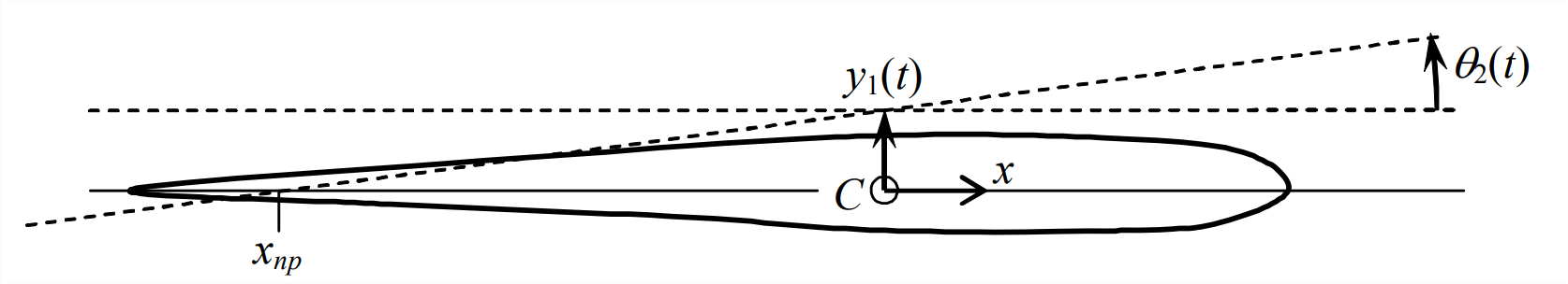
coordinate xnp shown at the intersection of the static equilibrium chord line and the displaced chord line is the nodal point. Using the geometry of small rotation and the notation on Figure \(\PageIndex{2}\), we have \(y_{1}(t) \approx-x_{n p} \theta_{2}(t)\); the minus sign is necessary because \(x_{n p}\) as shown is negative (aft of point \(C\)), but the values of \(y_{1}(t)\) and \(\theta_{2}(t)\) shown are positive. Therefore, the location of the nodal point for vibration mode \(n\) is given by

\[\left(x_{n p}\right)_{n}=-\frac{y_{1}(t)}{\theta_{2}(t)}=-\frac{Y_{1 n}}{\Theta_{2 n}}\label{eqn:12.30} \]

If mode \(n\) is mostly translation, with little rotation, then the coordinate might have such a large magnitude that there is no motionless point along the chord of the airfoil. However, if there is a nodal point on a typical section in a vibration test, one can easily observe it by sprinkling a little sand on the airfoil in the vicinity of the nodal point. As the body vibrates, the sand will migrate away from oscillating surfaces and accumulate on the motionless nodal point.

Rather than deal with an excessive number of algebraic symbols in equations such as Equation \(\ref{eqn:12.28}\), it is convenient now to consider a numerical example. A certain wind-tunnel typical section has a chord of 12 inches, weighs \(mg\) = 5.00 lb, has rotational “weight” about its mass center \(J_{C} g\) = 90.0 lb-inch², and has its mass center located \(r\) = 3.00 inches forward of the axis at which it is supported by lightweight flexible beams that function as springs. The spring constants provided by the beams are \(k_{y}\) = 51.0 lb/inch and \(k_\theta\) = 920 lb-inch/radian. The MATLAB session printed below evaluates Equations \(\ref{eqn:12.28}\) through \(\ref{eqn:12.30}\) for this numerical case.

» mg=5.00;Jcg=90.0;r=3.00;g=386.1; %mass and inertia constants

» ky=51.0;kt=920;format short e %stiffness constants

» p=[mg*Jcg/g^2 -(mg*(kt+ky*r^2)+Jcg*ky)/g ky*kt] %coeffs of Eq.(12-28)

p =

3.0187e-003 -2.9746e+001 4.6920e+004

» w_sqrd=roots(p) %roots w^2 of quadratic Eq.(12-28)

w_sqrd =

7.8822e+003

1.9720e+003

» wn=[sqrt(w_sqrd(2)) sqrt(w_sqrd(1))] %circular natural frequencies (in rad/s) arranged in ascending order

wn =

4.4407e+001 8.8782e+001

» fn=wn/2/pi %cyclic natural frequencies (in Hz)

fn =

7.0676e+000 1.4130e+001

» Th2n=(ky-mg/g*wn.^2)/(r*ky) %Eq.(12-29) for mode shape components \(\Theta\)2n, with Y1n = 1 inch

Th2n =

1.6642e-001 -3.3382e-001

» XNPn=(-1)./Th2n %Eq.(12-30) for locations of the nodal points

The numerical results of the MATLAB calculations are summarized in the following table:

Mode of vibration \(n\)	1	2
Natural frequency \(\omega_n\) and \(f_n=\omega_n/2 \pi\)	\(\omega_1\) = 44.41 rad/s \(f_1\) = 7.068 Hz	\(\omega_2\) = 44.41 88.78 rad/s \(f_2\) = 14.13 Hz
Mode shape	\(\left[\begin{array}{l} Y_{11} \\ \Theta_{21} \end{array}\right]=\left[\begin{array}{c} 1 \text { inch } \\ 0.1664 \mathrm{rad} \end{array}\right]\)	\(\left[\begin{array}{c} Y_{12} \\ \Theta_{22} \end{array}\right]=\left[\begin{array}{c} 1 \text { inch } \\ -0.3338 \mathrm{rad} \end{array}\right]\)
Nodal point location \(\left(x_{n p}\right)_{n}\)	−6.01 inch	+3.00 inch

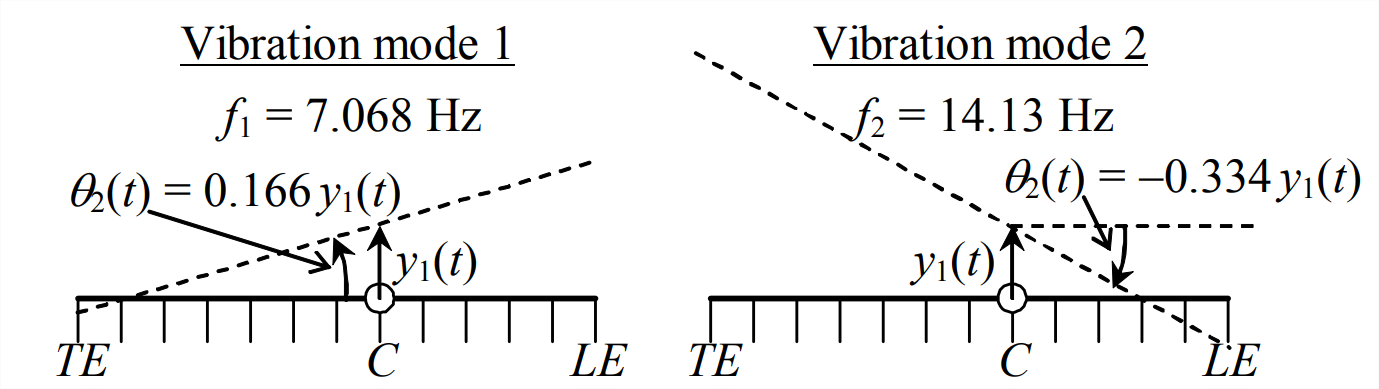
The vibration modes of this typical section are also displayed effectively in a graphical format, Figure \(\PageIndex{3}\), which is comparable to Figure 12.2.2 for the mass-spring system. Figure \(\PageIndex{3}\) indicates the airfoil in its reference position with a solid chord line, and in a modal displaced position with a dashed chord line. Let us suppose that mass center \(C\) is located 5 inches aft of leading edge LE along the 12-inch chord. In this case, the nodal points of both modes (listed in the table above) are located on the airfoil as shown on Fig. 12-6, not forward of \(LE\) or aft of trailing edge \(TE\). For graphical clarity, the magnitudes of motions \(y_{1}(t)\) and \(\theta_{2}(t)\) are shown greatly exaggerated relative to the 12-inch chord. Actual motions of a realistic typical section would be tens or hundreds of times smaller.

Figure \(\PageIndex{3}\): Vibration modes of the example typical section