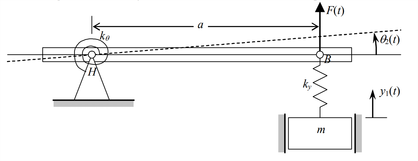
Consider again the 2-DOF system of homework Problem 11.2, depicted below.
Figure \(\PageIndex{1}\)
The two coupled differential equations of motion for this system, as derived for homework Problem 11.2 and now expressed in matrix form, are \[\left[\begin{array}{cc}
m & 0 \\
0 & J_{H}
\end{array}\right]\left[\begin{array}{c}
\ddot{y}_{1} \\
\ddot{\theta}_{2}
\end{array}\right]+\left[\begin{array}{cc}
k_{y} & -a k_{y} \\
-a k_{y} & k_{\theta}+a^{2} k_{y}
\end{array}\right]\left[\begin{array}{c}
y_{1} \\
\theta_{2}
\end{array}\right]=\left[\begin{array}{c}
0 \\
a F(t)
\end{array}\right] \nonumber \]All the parameters in these equations are defined on the figure except \(J_H\), which is the rotational inertia of the bar about frictionless hinge \(H\). Consider the free-vibration problem, with \(F(t)=0\). First, show that the characteristic equation in general is \[m J_{H}\left(\omega^{2}\right)^{2}+\left[-m\left(k_{\theta}+a^{2} k_{y}\right)-J_{H} k_{y}\right] \omega^{2}+k_{y} k_{\theta}=0 \nonumber \]Now, consider the following situation. Suppose that you are a design engineer working on a new satellite project for an aerospace company. You have designed a sensor package that includes a small mechanical device in the form of the subject 2-DOF system. The satellite has been fabricated, and is now being subjected to functional ground testing. The primary attitude-control actuator for the satellite is a control-moment gyroscope (CMG), the rotor of which spins at 11,400 rpm in normal operation. The spin-up time for this CMG is about four hours. During the first functional test, at the very end of the CMG spin-up, test engineers observe a short period of loud buzzing coming from the vicinity of your sensor package. The buzzing suddenly stops, and nobody thinks anything more about it until functional tests begin on your sensor. Unfortunately, the readings from your sensor are gibberish. The sensor package is removed and opened up, and examination shows that the 2-DOF device is completely destroyed: both springs are fractured, the bar is badly bent, the mass is detached, and the bar and mass have banged against near-by circuit boards within the package. It is now your responsibility to determine what went wrong. One experienced test engineer speculates that the 2-DOF device might have resonated due to base excitation caused by the CMG. Although the rotors of space-qualified CMGs are always carefully balanced, it is impossible to remove all imbalance. Consequently, rotor-spin imbalance imposes small periodic forces at the spin rate onto the CMG supports, and these forces produce vibration that is transmitted in waves throughout the spacecraft structure. With the assistance of calibration technicians, you determine that the numerical parameters of the 2-DOF device are: \(m\) = 19.2 g = 0.0192 kg, \(J_{H}\) = 37.3e−6 kg-m2, \(k_{y}\) = 16.9 N/mm = 16.9 kN/m, \(k_{\theta}\) = 12.8 N-m/rad, and \(a\) = 30.0 mm = 0.0300 m. Calculate the vibration modes of this system (natural frequencies, mode shapes, and sketches of the mode shapes), and discuss in a few sentences the probable cause of the structural failure within your satellite sensor package.
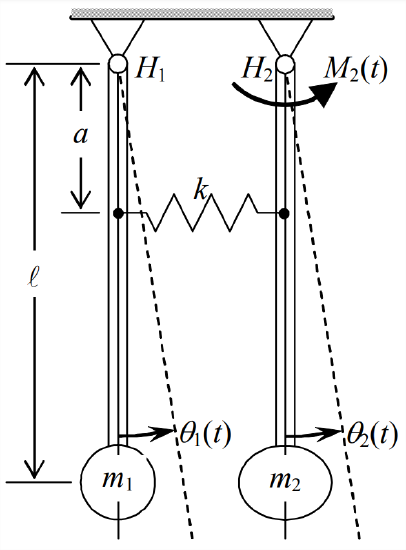
Consider again the 2-DOF pendulum-spring system of homework Problem 11.5, depicted below. The two coupled differential equations of motion for this system, as derived for homework Problem 11.5 and now expressed in matrix form, are \[\left[\begin{array}{cc}
m_{1} \ell^{2} & 0 \\
0 & m_{2} \ell^{2}
\end{array}\right]\left[\begin{array}{c}
\ddot{\theta}_{1} \\
\ddot{\theta}_{2}
\end{array}\right]+\left[\begin{array}{cc}
m_{1} g \ell+k a^{2} & -k a^{2} \\
-k a^{2} & m_{2} g \ell+k a^{2}
\end{array}\right]\left[\begin{array}{c}
\theta_{1} \\
\theta_{2}
\end{array}\right]=\left[\begin{array}{c}
0 \\
M_{2}(t)
\end{array}\right] \nonumber \]Consider the free-vibration problem, with \(M_{2}(t)=0\). It will simplify the writing if, initially, you will use the following notational abbreviations: \(J_{1}=m_{1} \ell^{2}\), \(J_{2}=m_{2} \ell^{2}\), \(k_{1}=m_{1} g \ell+k a^{2}\), \(k_{2}=m_{2} g \ell+k a^{2}\), and \(k_c=k a^{2}\) (the “coupling” coefficient). First, show that the characteristic equation in general is\[J_{1} J_{2}\left(\omega^{2}\right)^{2}+\left(-J_{2} k_{1}-J_{1} k_{2}\right) \omega^{2}+k_{1} k_{2}-k_{c}^{2}=0 \nonumber \]Now consider the special case with \(m_{1}=\frac{1}{2} m_{2}\) and \(k_c=k a^{2}=m_{2} g \ell\). Express all the coefficients of the characteristic equation in terms of \(m_2\), \(g\), and \(\ell\), and then show that this quadratic equation can be put into the form \(\left(\omega^{2}\right)^{2}-5(g / \ell) \omega^{2}+4(g / \ell)^{2}=0\). For this special case, solve for the natural frequencies and mode shapes, and sketch the mode shapes.
Figure \(\PageIndex{2}\)
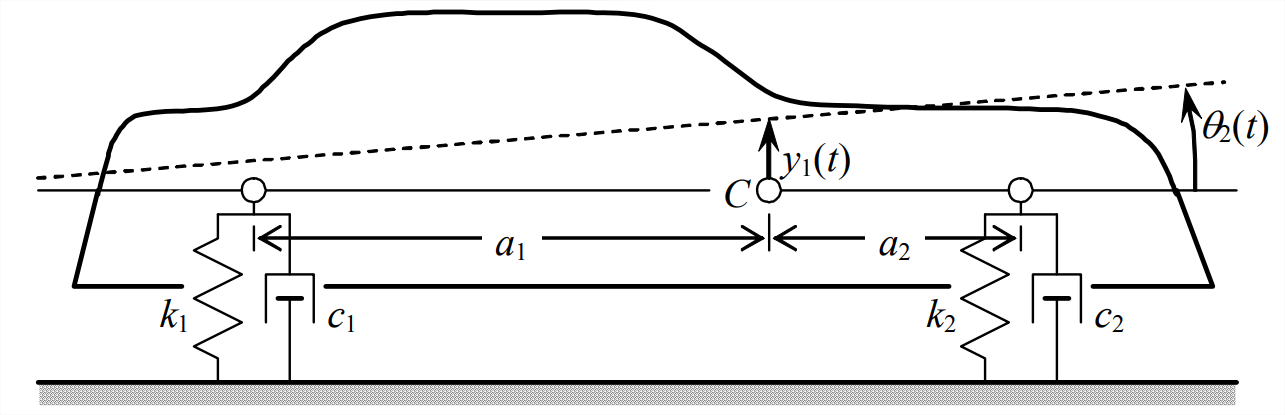
Consider again from homework Problem 11.6 the simplified model for pitching-translation dynamics of an automotive vehicle, depicted below. The rigid body frame has mass \(m\) and rotational inertia \(J_c\) about center of mass \(C\).
Figure \(\PageIndex{3}\)
The two coupled differential equations of motion for this system, as derived for homework Problem 11.6 and now expressed in matrix form, are\[\left[\begin{array}{cc}
m & 0 \\
0 & J_{C}
\end{array}\right]\left[\begin{array}{c}
\ddot{y}_{1} \\
\ddot{\theta}_{2}
\end{array}\right]+\left[\begin{array}{cc}
c_{1}+c_{2} & c_{2} a_{2}-c_{1} a_{1} \\
c_{2} a_{2}-c_{1} a_{1} & c_{1} a_{1}^{2}+c_{2} a_{2}^{2}
\end{array}\right]\left[\begin{array}{c}
\dot{y}_{1} \\
\dot{\theta}_{2}
\end{array}\right]+\left[\begin{array}{c}
k_{1}+k_{2} \\
k_{2} a_{2}-k_{1} a_{1}
\end{array} \quad \begin{array}{c}
k_{2} a_{2}-k_{1} a_{1} \\
k_{1} a_{1}^{2}+k_{2} a_{2}^{2}
\end{array}\right]\left[\begin{array}{c}
y_{1} \\
\theta_{2}
\end{array}\right]=\left[\begin{array}{c}
0 \\
0
\end{array}\right] \nonumber \]To obtain the vibration modes of the undamped system, we set \(c_{1}=c_{2}=0\), which deletes the entire second term of the matrix equation. The following data are representative for a compact four-door sedan: \(mg\) = 2,150 lb, \(J_cg\) = 5.47e6 lb-inch2, \(k_{1}=k_{2}=\) 155 lb/inch, \(a_{1}=82.7\) inches, and \(a_{2}=35.4\) inches. Calculate the natural frequencies, mode shapes, and nodal point locations, and sketch the mode shapes.
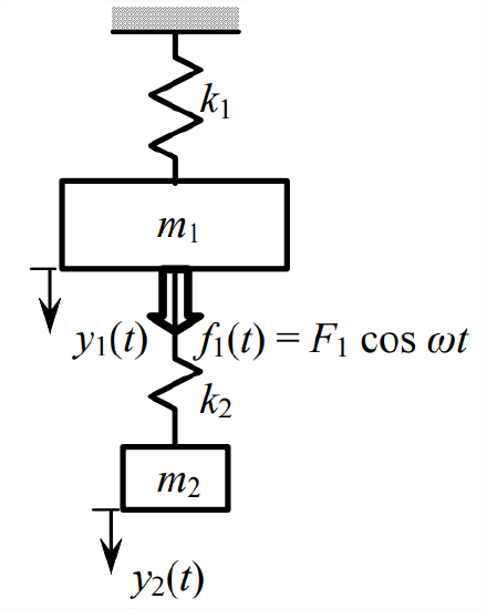
Consider again Figure 12.2.1, but now suppose that the entire undamped mass-spring system consists of a primary sub-system, with mass \(m_1\) and spring \(k_1\), plus a smaller auxiliary sub-system, with mass \(m_2\) and spring \(k_2\); also, that a steady sinusoidal force \(f_{1}(t)=F_{1} \cos \omega t\) acts upon \(m_1\), but no externally applied force acts upon \(m_2\), \(f_2(t) = 0\). Your assignment is to solve for and evaluate the steady-state forced sinusoidal responses \(y_{1}(t)=Y_{1}(\omega) \cos \omega t\) and \(y_{2}(t)=Y_{2}(\omega) \cos \omega t\). To solve, use the theory developed in Section 12.2, not the more general procedure described in Section 4.7 for finding frequency-response functions.
Figure \(\PageIndex{4}\)
Determine algebraic equations for \(Y_{1}(\omega)\) and \(Y_{2}(\omega)\) in terms of \(m_1\), \(k_1\), \(m_2\), \(k_2\), \(F_1\), and \(\omega\). Also, write the characteristic equation of the free-vibration problem, and explain what happens if its roots are substituted into the equations for \(Y_{1}(\omega)\) and \(Y_{2}(\omega)\).
Suppose that this is a system for which vibration isolation is required: primary mass \(m_1\) includes an unbalanced reciprocating motor or machine that oscillates with specific frequency \(\omega=\Omega\), which tends to cause \(m_1\) to vibrate vertically at frequency \(\omega\); but it is desirable to protect from that vibration the supporting structure to which primary spring \(k_1\) is attached. (See homework Problem 10.13 for additional discussion of vibration isolation.) According to your solution in part 12.4.1, what happens to motion amplitudes \(Y_{1}(\Omega)\) of \(m_1\) and \(Y_{2}(\Omega)\) of \(m_2\) if you tune the single-DOF frequency of the auxiliary mass and spring, \(m_2\) and \(k_2\), to the excitation frequency, i.e., if you design the auxiliary sub-system so that \(k_{2} / m_{2} \equiv \Omega^{2}\)? With \(k_{2} / m_{2} \equiv \Omega^{2}\), what is the sinusoidal force \(k_{2}\left[y_{2}(t)-y_{1}(t)\right]\) that spring \(k_2\) imposes on primary mass \(m_1\)? With the correct answers to these questions, you will have explained the functioning of an ideal undamped dynamic vibration absorber.
An ideal undamped dynamic vibration absorber is unattainable in reality because systems always have some damping. Moreover, even if we could magically eliminate all damping, the ideal absorber would still have a serious deficiency: if the excitation frequency were to differ from the nominal value, which usually happens in practice during motor start-up or off-nominal operation, then the system could experience a 2-DOF resonance failure. Suppose, for example, we have the following numerical parameters: \(m_1\) = 25.3 kg, \(k_1\) = 2.62 MN/m, \(\Omega / 2 / \pi\) = 50 Hz, and the auxiliary sub-system is tuned to 50 Hz with \(m_2\) = 5.066 kg and \(k_2\) = 0.5 MN/m. First, solve the characteristic equation to calculate the two system natural frequencies in Hz, \(f_{1}=\omega_{1} / 2 / \pi<f_{2}=\omega_{2} / 2 / \pi\); if you wish, you may use the roots MATLAB function for this task. Next, calculate and plot versus excitation frequency (in Hz) the frequency-response dynamic flexibility, \(Y_{1}(\omega) / F_{1}\), of the primary sub-system. The range of excitation frequencies over which you plot this response must include at least all three frequencies, \(f_1\), \(\omega⁄ 2⁄ \pi\), and \(f_2\); it probably should even extend somewhat below the lowest of these three and somewhat above the highest. Be sure to include appropriate axis labels on your graph. Your graph should display clearly both the strengths and the weaknesses of the ideal undamped dynamic vibration absorber for these particular numerical parameters.1
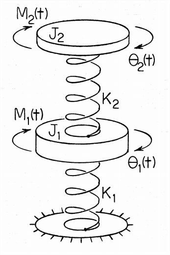
The drawing at right represents a rotational mechanical system that is directly analogous to the translational mechanical system of Figure 12.2.1. Rotational inertias \(J_1\) and \(J_2\) are analogous, respectively, to masses \(m_1\) and \(m_2\) on Figure 12.2.1; rotational springs \(K_1\) and \(K_2\) are analogous to translational springs \(k_1\) and \(k_2\); applied moments \(M_1(t)\) and \(M_2(t)\) are analogous to applied forces \(f_1(t)\) and \(f_2(t)\); and rotations \(\theta_1(t)\) and \(\theta_2(t)\) are analogous to translations \(y_1(t)\) and \(y_2(t)\). Therefore, the matrix equation of motion for this rotational system is directly analogous to Equation 12.2.3 for the translational system:
Figure \(\PageIndex{5}\)
\[\overbrace{\left[\begin{array}{cc}
J_{1} & 0 \\
0 & J_{2}
\end{array}\right]}^{\text{inertia matrix}}\left[\begin{array}{c}
\ddot{\theta}_{1} \\
\ddot{\theta}_{2}
\end{array}\right]+\overbrace{\left[\begin{array}{cc}
K_{1}+K_{2} & -K_{2} \\
-K_{2} & K_{2}
\end{array}\right]}^{\text{structural stiffness matrix}}\left[\begin{array}{c}
\theta_{1} \\
\theta_{2}
\end{array}\right]=\left[\begin{array}{c}
M_{1}(t) \\
M_{2}(t)
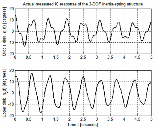
\end{array}\right] \nonumber \]Consider a 2-DOF inertia-spring system with rotational inertias \(J_{1}=J_{2}=0.01042\) kg-m2 and rotational stiffness constants \(K_{1}=K_{2}=2.77\) N-m/rad. Your assignment is to calculate and plot, over the time interval \(0 \leq t \leq 5\) seconds, the unforced initial-condition (IC) responses, rotations \(\theta_{1}(t)\) and \(\theta_{2}(t)\), of this system if the initial rotations are \(\theta_{1}(0)=\theta_{2}(0)=14.58\) degrees, and the initial rotational velocities are zero. Use the theory (and even the appropriate calculations, if you wish) of Section 12.2. The given inertias and stiffness constants are those of a real structural system, which is described on the next two pages, and the given initial conditions were imposed on that system, producing the measured responses shown on the graph following this paragraph. Your theoretical responses should appear somewhat similar to the measured responses, but the theoretical and measured responses should differ in one significant respect. Read the description below of the actual structural system, then identify the property of all real mechanical dynamic systems that is not modeled by the theory of Chapter 12, and explain how this modeling deficiency is illustrated in the differences between the theoretical and measured responses shown on the graphs.
Figure \(\PageIndex{6}\)
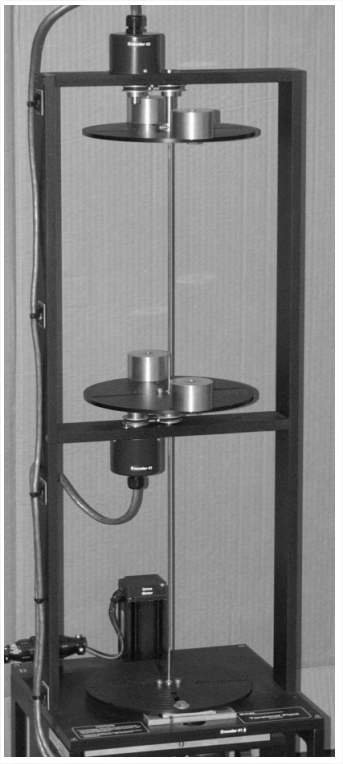
The photograph on the next page shows the relevant structural portion of the actual laboratory system2 that is represented by the drawing on the previous page, and from which the IC-response graph above was measured. Three steel disks are attached to a continuous steel shaft of diameter about 3.2 mm. Each disk is 20 cm in diameter and 0.5 cm thick, with four radial slots to accommodate added masses. The total length of shaft between lower and upper disks is about 68 cm. The shaft is supported near the middle and upper disks by bearings, which impose some damping on the structure. The lower disk is clamped to the frame, so the shaft is fixed at the bottom but is free to twist everywhere else along its length. Two metal cylinders, each of nominal mass 0.5 kg, are bolted symmetrically at 9-cm radii to each of the middle and upper disks. The rotational inertias of the two bulked-up disks are orders of magnitude greater than that of the shaft, so this system is effectively a 2-DOF rotational structure, those DOFs being rotations \(\theta_{1}(t)\) and \(\theta_{2}(t)\) of the middle and upper disks, respectively. \(\theta_{1}(t)\) and \(\theta_{2}(t)\) are sensed by the optical encoders shown on the photograph; each encoder shaft is connected to the structural shaft by a lightweight belt and pulleys, which add to the system some damping but negligible inertia.
A clever student determined experimentally the inertias and stiffness constants of this system, rather than relying on purely theoretical calculations, mostly by using the added-inertia method (from homework Problem 7.9). To determine \(J_2\) and \(K_2\), the student clamped the middle disk to the frame, and then measured free-vibration frequencies of the upper disk [\(\theta_2(t)\) with \(\theta_1(t) = 0\)], both bare and with symmetrically added combinations of the metal cylinders. The student determined \(J_1\) and \(K_1 + K_2\) by clamping the upper disk, and then measuring free-vibration frequencies of the middle disk [\(\theta_1(t)\) with \(\theta_2(t) = 0\)]. The values of the parameters determined by this process are \(J_{1}=J_{2}=0.01042\) (\(\pm 0.00003\)) kg-m2 and \(K_{1}=K_{2}=2.77\) (\(\pm 0.04\)) N-m /rad.
The initial rotations, \(\theta_{1}(0)=\theta_{2}(0)= 14.58^{\circ}\), were imposed on the middle and upper disks by twang, also known as snapback, excitation: a fine thread was tied around the front cylinder of the middle disk, the thread was pulled laterally and the opposite end was anchored, thus imposing onto the middle disk the static initial rotation, then the thread was cut with scissors, abruptly releasing the middle and upper disks to free vibration. The structural shaft was fixed only at the bottom, so the initial rotation of the upper disk was the same as that of the middle disk.
Figure \(\PageIndex{7}\)
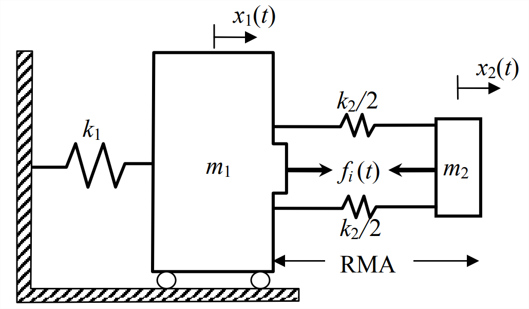
A structure’s fundamental mode of vibration is represented in the drawing below by mass \(m_1\) and spring \(k_1\), with the translation of \(m_1\) denoted as \(x_1(t)\). Suppose we wish to exercise active control over that vibration by use of an attachment to the structure: a reaction-mass actuator (RMA), represented in the diagram by reaction mass \(m_2\), spring \(k_2\), and internally generated force \(f_i(t)\) acting equally and oppositely on \(m_2\) and \(m_1\), with the translation of \(m_2\) denoted as \(x_2(t)\). (To simplify the equations here, we neglect the normally small natural passive damping inherent in both structures and RMAs.) Use Equation 12.2.3 to write the matrix equation of motion for this combination of structure and RMA. Next, revise this equation to include the particular type of feedback vibration control described in the following. Suppose that reaction mass \(m_2\) carries a transducer that senses the translational velocity of \(m_2\) relative to that of \(m_1\) and generates an electrical voltage signal proportional to that relative velocity, \(e_{v}(t)=V\left(\dot{x}_{2}-\dot{x}_{1}\right)\), where \(V\) is a calibration constant with units such as volt per meter/s. Homework Problem 10.15 explains that an external voltage signal \(e_i(t)\) [not shown on this drawing] commands internal force \(f_i(t)\) according to the linear relationship \(f_{i}(t)=G e_{i}(t)\), \(G\) being a constant with units such as newton per volt. Suppose that we multiply the relative velocity signal \(e_v(t)\) by a variable gain factor \(F\) (using, e.g., a non-inverting amplifier, homework Problem 5.8) and then feed the multiplied signal back to serve as the force-command signal, \(e_{i}(t)=F e_{v}(t)=F V\left(\dot{x}_{2}-\dot{x}_{1}\right)\). Therefore, the generated internal force is \(f_{i}(t)=G e_{i}(t)=G F V\left(\dot{x}_{2}-\dot{x}_{1}\right) \equiv C\left(\dot{x}_{2}-\dot{x}_{1}\right)\), where we define the overall feedback constant \(C ≡ GFV\) with units such as newton per meter/second. Revise your matrix equation of motion to reflect the feedback vibration control described here; in particular, show that the feedback produces an artificial viscous damping matrix, \(C\left[\begin{array}{cc}
1 & -1 \\
-1 & 1
\end{array}\right]\). With sufficiently large feedback gain factor \(F\) and sufficient authority of the RMA’s internal force generator, this form of control can impose significant positive damping upon a structure’s vibration.
Figure \(\PageIndex{8}\)
NOTE: It is not in required in this problem, but it might be of interest to you that replacing dependent variable \(x_2(t)\) with the relative translation of reaction mass \(m_2\), \(z(t) = x_2(t) − x_1(t)\) can transform the matrix equation of motion into the following form, in which the inertia matrix becomes full and symmetric, but the artificial damping and stiffness matrices become simpler and diagonal:\[\left[\begin{array}{cc}
m_{1}+m_{2} & m_{2} \\
m_{2} & m_{2}
\end{array}\right]\left[\begin{array}{c}
\ddot{x}_{1} \\
\ddot{z}
\end{array}\right]+\left[\begin{array}{cc}
0 & 0 \\
0 & C
\end{array}\right]\left[\begin{array}{c}
\dot{x}_{1} \\
\dot{z}
\end{array}\right]+\left[\begin{array}{cc}
k_{1} & 0 \\
0 & k_{2}
\end{array}\right]\left[\begin{array}{c}
x_{1} \\
z
\end{array}\right]=\left[\begin{array}{l}
0 \\
0
\end{array}\right] \nonumber \]
1Homework Problem 12.4 is only an introduction to the subject of dynamic vibration absorbers. See Den Hartog, 1956, Sections 3.2 and 3.3, for a more advanced and extensive treatment of this subject.
2This is a Model 205a Torsional Plant designed and fabricated by Educational Control Products of Bell Canyon, California, USA.