14.1: Initial Definitions and Terminology

As an introduction to feedback control and related matters, this chapter considers a common task for many engineering systems: remote (indirect) control of the rotational position of some solid body; let us refer to this solid body generically as the rotor. The input to a rotation-control system is typically a command issued by a human operator using a device such as a steering wheel, control column, dial, computer keyboard, etc.; the input can also be a computer-generated signal that carries previously programmed instructions. The output is the rotational position of the rotor. The modifiers “remote” and “indirect” of “control” mean that there is no direct, rigid, mechanical linkage between the input device and the rotor; instead, for a remote control system, there might exist between the input device and the rotor such engineering equipment as sensors, electrical circuits, signal processors (analog and/or digital), flexible links or cables, electromagnetic or acoustic transmitters and receivers, and actuators of many types (motors, thrusters, etc.).

The following are a few of the many “rotors” in modern engineering practice with which you are probably familiar: aerodynamic and hydrodynamic control surfaces, such as rudders, elevators, and ailerons; the steering mechanisms that guide land vehicles and taxiing airplanes; nozzles of rocket engines or vectored-thrust jet engines; any entire vehicle itself, the three-dimensional rotational orientation (roll, pitch, yaw) of which is generally called the vehicle’s attitude. You can probably add other rotors to this list from your own experience.

In general, the mass center of a solid body can have three degrees of rotational freedom. However, in order to keep the rotational dynamics simple here and to focus on feedback control, we will restrict our attention to rigid rotors that rotate in a plane about a fixed point, so that there is only one degree of rotational freedom.

Consider the simple generic rotor shown in Figure \(\PageIndex{1}\). Let us specify that it is restricted to rotating about the shaft axis, that its rotation angle relative to some reference position is \(\theta(t)\), and that its angular velocity is \(p(t) \equiv \dot{\theta}\). The rotational inertia of the rotor about the axis of rotation is denoted as \(J\), and the total moment applied onto the rotor by all sources is denoted as \(M(t)\). This is the physical object that we wish to control; in the terminology of control, the object or process to be controlled is often called the plant.

Figure \(\PageIndex{1}\): Generic rotor, the plant. (Copyright; author via source)

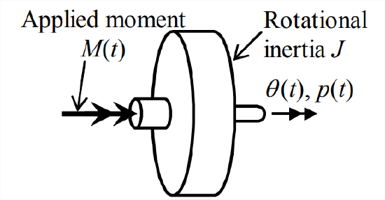
Provided that there is no damping moment proportional to \(p(t)\) imposed upon the rotor, the equation of motion for the plant of Figure \(\PageIndex{1}\) is a simplified version of Equation 3.3.2:

\[J \dot{p}=J \ddot{\theta}=M(t)\label{eqn:14.1} \]

Let us derive the transfer function of the plant, \(PTF(s)\), by taking the Laplace transform of Equation \(\ref{eqn:14.1}\) with zero initial conditions:

\[J s^{2} L[\theta(t)]=L[M(t)] \Rightarrow \operatorname{PTF}(s) \equiv \frac{L[\theta(t)]}{L[M(t)]}=\frac{1}{J s^{2}}\label{eqn:14.2} \]

In our previous work, we usually assumed that \(M(t)\) is known, and we then solved for the resulting \(p(t)\) and/or \(\theta (t)\). Now, our objective is different: for control, we want to command a desired rotor-position time history. The command usually is something like a steering-wheel position or dial setting, or a signal carrying computer-generated instructions. In order to distinguish the input command from the output rotor angle, we introduce a different symbol for the command:

\[r(t) \equiv \text { operator setting intended to produce the desired } \theta(t)\label{eqn:14.3} \]

Operator setting \(r(t)\) is the reference input quantity, which is transmitted to the system by electrical circuitry, mechanical linkages or cables, electromagnetic or acoustic waves, etc.