14.3: Closed-Loop Control of Rotor Position (1)

Let us modify the open-loop control system of Figure 14.2.1 in the following manner: measure the output with a rotational-position sensor, and send the voltage output from this sensor back to a summing junction that forms the error signal, which is the difference between the signal representing the operator setting and the signal representing the actual output. The feedback branch and summing junction convert the open-loop system into the closed-loop system depicted on Figure \(\PageIndex{1}\).

Figure \(\PageIndex{1}\): Functional diagram of position-feedback control system. (Copyright; author via source)

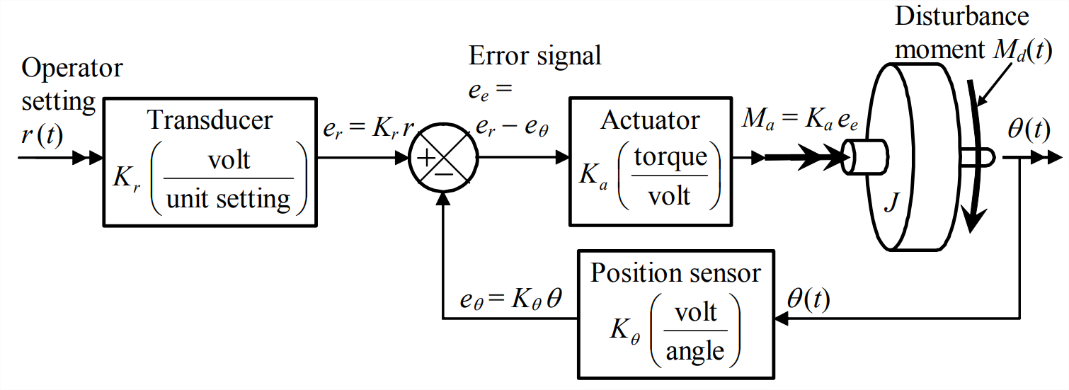
The elements of the closed-loop system are the same as those of the open-loop system, Figure 14.2.1, but with the addition of the output sensor and the summing junction (defined in Section 13.2). We assume that the sensor is a device such as an optical encoder, with accurately calibrated positive sensitivity \(K_{\theta}\) (volt per degree or radian). The summing junction could be a simple circuit consisting of an inverting amplifier (Figure 5.3.2) and a summing inverting amplifier (homework Problem 5.7).

This closed-loop system tends to be self-correcting. We can understand this tendency by writing in detail the equation for the control moment, from the signals labeled on Figure \(\PageIndex{1}\):

\[M_{a}(t)=K_{a} e_{e}(t)=K_{a}\left[e_{r}(t)-e_{\theta}(t)\right]=K_{a}\left[K_{r} r(t)-K_{\theta} \theta(t)\right]\label{eqn:14.11} \]

From Equation \(\ref{eqn:14.11}\), the control moment is zero when \(K_{r} r(t)-K_{\theta} \theta(t)=0\), so that

\[\theta(t)=\frac{K_{r}}{K_{\theta}} r(t)\label{eqn:14.12} \]

Equation \(\ref{eqn:14.12}\) clearly is the desired instantaneous linear relation of output \(\theta(t)\) to input \(r(t)\). At instants when Equation \(\ref{eqn:14.12}\) is not satisfied, the control actuator imposes a corrective moment. Suppose, for example, that at a certain instant both \(\theta(t)\) and \(r(t)\) are positive, but that the output is less than the desired value, \(\theta(t)<\left[K_{r} / K_{\theta}\right] r(t)\); at this instant, then, the error signal is \(K_{r} r(t)-K_{\theta} \theta(t)=e_{e}(t)>0\), and \(M_{a}(t)=K_{a} e_{e}(t)>0\) thus, when the output is less than it ought to be, the closed-loop control system imposes a positive moment to increase the output. Moreover, by reversing the inequality signs above, you can show that the control system imposes a negative moment to decrease the output when the output is greater than it ought to be.

Because the corrective moment is proportional to the output error and is independent of the theoretical model, the self-correcting tendency of this closed-loop control system is in effect regardless of how well the theoretical model represents the system and its environment.

To infer more information about the closed-loop system of Figure \(\PageIndex{1}\), let us derive the ODE of motion by substituting Equation \(\ref{eqn:14.11}\) into Equation 14.2.1:

\[J \ddot{\theta}=M_{a}(t)+M_{d}(t)=K_{a}\left[K_{r} r(t)-K_{\theta} \theta(t)\right]+M_{d}(t) \nonumber \]

\[\Rightarrow \quad J \ddot{\theta}+K_{a} K_{\theta} \theta=K_{a} K_{r} r(t)+M_{d}(t)\label{eqn:14.13} \]

From Equation \(\ref{eqn:14.13}\), we make the following observations:

1. the feedback control in Figure \(\PageIndex{1}\) has the effect of attaching between the operator setting and the rotor inertia an artificial restoring spring with stiffness constant \(K_{a} K_{\theta}\);
2. if only operator input \(r(t)\) acts, i.e., if \(M_{d}(t)=0\), then the desired output Equation \(\ref{eqn:14.12}\) is actually the pseudo-static response of the system (as defined in Section 7.1),\[K_{a} K_{\theta} \theta_{p s}=K_{a} K_{r} r(t) \Rightarrow \theta_{p s}(t)=\frac{K_{r}}{K_{\theta}} r(t)\label{eqn:14.14} \]
3. if only operator input \(r(t)\) acts, and if the input-transducer sensitivity equals the output-sensor sensitivity, \(K_{r}=K_{\theta}\), then the closed-loop system is directly analogous to an undamped, base-excited mass-spring system [as described by Equation 13.2.1 with \(c = 0\)];
4. the self-correcting tendency even counteracts the adverse influence of many types of disturbance, which we can conclude from our previous experience with forced-response solutions for 2^nd order systems.

If, for example, the disturbance is time-limited, such as a pulse, then post-pulse response due to the pulse will oscillate about zero but will not contain any constant steady-state component. If, for another example, the disturbance is sinusoidal, then the resulting response will oscillate about zero but will not contain any constant steady-state component; however, we can also see that if the frequency of the sinusoidal disturbance is in the neighborhood of the closed-loop system natural frequency, \(\omega_{n}=\sqrt{K_{a} K_{\theta} / J}\), then the disturbance could produce resonance, which this particular control system could not prevent.

To establish the method for analysis later of more complicated control systems, let us draw and analyze the Laplace block diagram corresponding to functional diagram Figure \(\PageIndex{1}\). For this task, we define the following Laplace transforms: \(L[r(t)] \equiv R(s)\), \(L[\theta(t)] \equiv \Theta(s)\), \(L\left[e_{r}(t)\right] \equiv E_{r}(s)\), \(L\left[e_{\theta}(t)\right] \equiv E_{\theta}(s)\), \(L\left[e_{e}(t)\right] \equiv E_{e}(s)\), \(L\left[M_{a}(t)\right] \equiv \mathrm{M}_{\mathrm{a}}(s)\), \(L\left[M_{d}(t)\right] \equiv \mathrm{M}_{\mathrm{d}}(s)\), and \(L[M(t)] \equiv \mathrm{M}(s)\). The Laplace block diagram, Figure \(\PageIndex{2}\), is similar to the functional diagram, except that we replace the rotor in Figure \(\PageIndex{1}\) with its transfer function, \(P T F(s)\) of Equation 14.1.2, and we use a summing junction to denote the actions upon the rotor of both control moment \(M_{a}(t)\) and disturbance moment \(M_{d}(t)\).

Figure \(\PageIndex{2}\): Laplace block diagram, including disturbance input, of position-feedback control system. (Copyright; author via source)

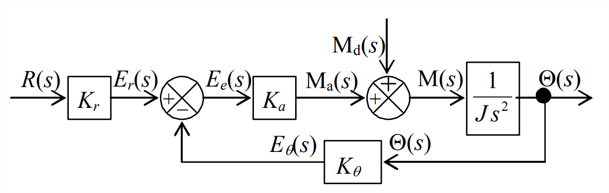
This system actually has two independent inputs, \(r(t)\) and \(M_d(t)\), so it is not strictly a single-input-single-output (SISO) system. However, the most important fundamental relationship for this control system is that between the reference input and output \(\theta(t)\), so we now will focus on that relationship by setting \(M_{d}(t)=0\). Therefore, \(\mathrm{M}_{\mathrm{d}}(s)=0\), and we re-draw Figure \(\PageIndex{2}\) as the SISO block diagram at right, with the objective of deriving from it the closed-loop transfer function, \(\operatorname{CLTF}(s) \equiv \Theta(s) / R(s)\).

Figure \(\PageIndex{3}\): Laplace block diagram of SISO position-feedback control system. (Copyright; author via source)

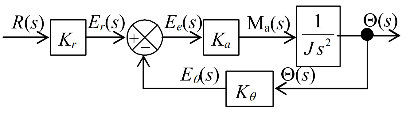
Three distinct steps of block-diagram algebra are required to reduce Figure \(\PageIndex{3}\) to a single block, the \(\operatorname{CLTF}(s)\), that separates input and output signals:

1. Combine (multiply) the two block transfer functions within the forward branch of the loop, as shown below. This multiplication operation is derived in Section 13.1.

   

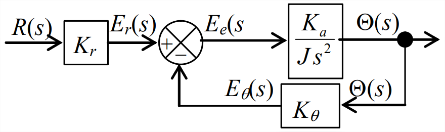
   Figure \(\PageIndex{4}\): Step 1. (Copyright; author via source)

2. Resolve the forward-branch and feedback-branch transfer functions of the closed loop into the single equivalent transfer function shown below. The block-diagram algebra used in this step is derived in the next section; it is an important basic tool for the analysis of control systems.

   

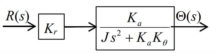
   Figure \(\PageIndex{5}\): Step 2. (Copyright; author via source)

3. Finally, and obviously, just multiply the remaining two blocks to produce the required result shown below.

   

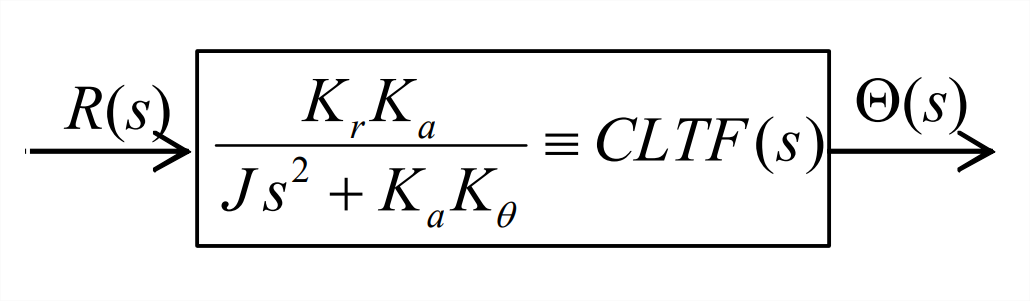
   Figure \(\PageIndex{6}\): Step 3. (Copyright; author via source)

For this relatively simple system, the SISO version of ODE of motion Equation \(\ref{eqn:14.13}\) is \(J \ddot{\theta}+K_{a} K_{\theta} \theta=K_{a} K_{r} r(t)\). It is very easy to derive the same \(\operatorname{CLTF}(s)\) directly from this ODE, but we have derived \(\operatorname{CLTF}(s)\) here using block-diagram algebra in order to establish the approach that is appropriate for more complicated systems.

We shall re-visit this position-feedback control system in Section 14.5, with the objectives of evaluating its control performance and then developing an addition to the systems that will improve the performance.