14.4: Transfer Function of a Single Closed Loop

Consider Figure \(\PageIndex{1}\), which is a more general version, in standard notation, of the closed loop in Figure 14.3.4. General functions \(G(s)\) and \(H(s)\) are, respectively, the forward-branch and feedback-branch transfer functions. \(E(s)\) is the actuating error signal, and \(B(s)\) is the feedback signal. We seek the closed-loop transfer-function, the ratio \(\operatorname{Out}(s) / \operatorname{In}(s)\).

Figure \(\PageIndex{1}\): Laplace block diagram of general closed loop. (Copyright; author via source)

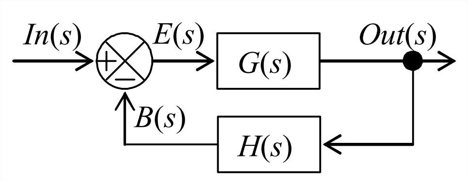
All of the quantities labeled on Figure \(\PageIndex{1}\) are denoted as functions of Laplace variable \(s\), but it is important to recognize that there are two fundamentally different types of functions:

1. the “signals” \(\operatorname{In}(s)\), \(E(s)\), \(B(s)\), and \(\operatorname{Out}(s)\), which actually are Laplace transforms of time-dependent variables such as motion and voltage; and
2. the transfer functions \(G(s)\) and \(H(s)\), which represent in the Laplace domain the characteristics of systems and objects such as inertia and circuits. To emphasize the difference in the following derivation of \(\operatorname{Out}(s) / \operatorname{In}(s)\), let us omit the functional notation “(\(s\))” from the signals, at least in the intermediate steps. The steps follow naturally from Figure \(\PageIndex{1}\):

\[E=I n-B \quad \text { and } \quad B=O u t \times H(s), \nonumber \]

\[\Rightarrow \quad O u t=E \times G(s)=[\operatorname{In}-B] \times G(s)=[\operatorname{In}-O u t \times H(s)] \times G(s) \nonumber \]

\[=\operatorname{In} \times G(s)-O u t \times H(s) \times G(s) \nonumber \]

\[\Rightarrow \quad O u t \times[1+G(s) H(s)]=\operatorname{In} \times G(s) \nonumber \]

\[\Rightarrow \frac{O u t(s)}{\operatorname{In}(s)}=\frac{G(s)}{1+G(s) H(s)}\label{eqn:14.15} \]

Equation \(\ref{eqn:14.15}\) is an important, general, labor-saving tool for analysis of loops in any control system, not just the systems discussed in this chapter. To illustrate its application, let us use it to derive in detail the loop transfer function written in Step 2 of the block-diagram algebra of Section 14.3. From Step 1 of that process (or from Figure 14.3.4), we identify: \(G(s)=K_{a} / J s^{2}\) and \(H(s)=K_{\theta}\). Substituting these into Equation \(\ref{eqn:14.15}\) gives \(\frac{\operatorname{Out}(s)}{\operatorname{In}(s)}=\frac{K_{a} / J s^{2}}{1+\left(K_{a} / J s^{2}\right) K_{\theta}}=\frac{K_{a}}{J s^{2}+K_{a} K_{\theta}}\), which is the loop transfer function shown in the block diagram as the result of Step 2.

A transfer function in Equation \(\ref{eqn:14.15}\) often has the form of a ratio of polynomials in \(s\), such as \(G(s)\) in the previous paragraph, so it is useful to derive a version of Equation \(\ref{eqn:14.15}\) in terms of the polynomials. First, we define numerator and denominator polynomials that make up \(G(s)\) and \(H(s)\):

\[G(s) \equiv \frac{N_{G}(s)}{D_{G}(s)} \text { and } H(s) \equiv \frac{N_{H}(s)}{D_{H}(s)}\label{eqn:14.16} \]

Next, we carry out the algebra of Equation \(\ref{eqn:14.15}\), dropping the functional notation "(\(s\))" from the transfer functions and polynomials in the interest of notational conciseness:

\[\frac{O u t(s)}{\operatorname{In}(s)}=\frac{G}{1+G H}=\frac{N_{G} / D_{G}}{1+\left(N_{G} / D_{G}\right) \times\left(N_{H} / D_{H}\right)}=\frac{N_{G} D_{H}}{D_{G} D_{H}+N_{G} N_{H}}\label{eqn:14.17} \]

For the example of the previous paragraph, the simple polynomials are \(N_{G}=K_{a}\), \(D_{G}=J_{S}^{2}\), \(N_{H}=K_{\theta}\), and \(D_{H}=1\); substituting these terms into Equation \(\ref{eqn:14.17}\) obviously leads to the, \(\operatorname{Out}(s) / \operatorname{In}(s)\) result derived in the previous paragraph, but with a bit less algebra because the algebra has been completed in Equation \(\ref{eqn:14.17}\). Equation \(\ref{eqn:14.17}\) expresses the closed-loop transfer function as a ratio of polynomials, and it applies in general, not just to the problems of this chapter.

Finally, we will use later an even more specialized form of Equations \(\ref{eqn:14.15}\) and \(\ref{eqn:14.17}\) for the case of unity feedback, \(H(s)=1=1 / 1\):

\[\frac{\operatorname{Out}(s)}{\operatorname{In}(s)}=\frac{G}{1+G}=\frac{N_{G}}{D_{G}+N_{G}}\label{eqn:14.18} \]

Equations \(\ref{eqn:14.15}\), \(\ref{eqn:14.17}\), and \(\ref{eqn:14.18}\) are very useful for the analysis of feedback control. In the future, whenever you encounter a simple loop with the form of Figure \(\PageIndex{1}\) in the Laplace block diagram of a system, you may (and usually should) apply whichever of these equations is most appropriate to derive the loop transfer function, without repeating the algebra that goes into the derivation of these equations.