
14.5: Closed-Loop Control of Rotor Position (2)
- Page ID
- 7716

Let us re-visit the position-feedback control system of Section 14.3 in order, first, to evaluate its control performance and, next, to develop an addition to the system that will improve the performance.
It is easy to evaluate the control performance just by considering the SISO version of ODE of motion Equation 14.3.4, which is
\[J \ddot{\theta}+K_{a} K_{\theta} \theta=K_{a} K_{r} r(t)\label{eqn:14.19} \]
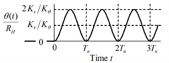
As was noted earlier, the pseudo-static response of Equation \(\ref{eqn:14.19}\) is \(\theta_{p s}(t)=\left[K_{r} / K_{\theta}\right] r(t)\); this would be good controlled response, but it is not necessarily the total response. Therefore, let us consider in more detail the total transient response. Equation \(\ref{eqn:14.19}\) is an undamped 2nd order ODE of the type analyzed extensively in Chapter 7. By dividing Equation \(\ref{eqn:14.19}\) through by \(J\) and then defining appropriate parameters, we can adapt this ODE to the standard form Equation 7.1.5, \(\ddot{\theta}+\omega_{n}^{2} \theta=\omega_{n}^{2} u(t)\), in which the natural frequency is \(\omega_{n}=\sqrt{K_{a} K_{\theta} / J}\), and the standard input quantity is \(u(t)=\left[K_{r} / K_{\theta}\right] r(t)\). We can also adapt any appropriate response solutions already derived in Chapters 7 and 8 to this position-feedback control system. For example, if the operator setting is the step function \(r(t)=R_{H} H(t)\), then \(u(t)=\left[K_{r} / K_{\theta}\right] R_{H} H(t) \equiv U H(t)\), so the standard solution Equation 7.3.8 leads to step response \(\theta(t)=\left(K_{r} / K_{\theta}\right) R_{H}\left(1-\cos \omega_{n} t\right)\). This step response is plotted on the figure at right, with the period defined as \(T_{n}=2 \pi / \omega_{n}\). Due to the absence of damping, the response oscillates forever about the desired constant pseudo-static response, \(\theta_{p s}=\left(K_{r} / K_{\theta}\right) R_{H}\). The response never settles at \(\theta_{p s}\), so the control system fails to deliver the desired performance.
We must conclude from this example that the absence of damping renders the position-feedback control system of Section 14.3 (Figure 14.3.1) unsuitable for most, if not all engineering applications of control. However, there is a relatively simple design feature that can be added to the control system, a feature that will provide damping to the system and will greatly improve the control performance.
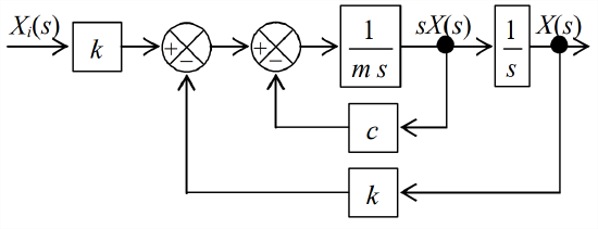
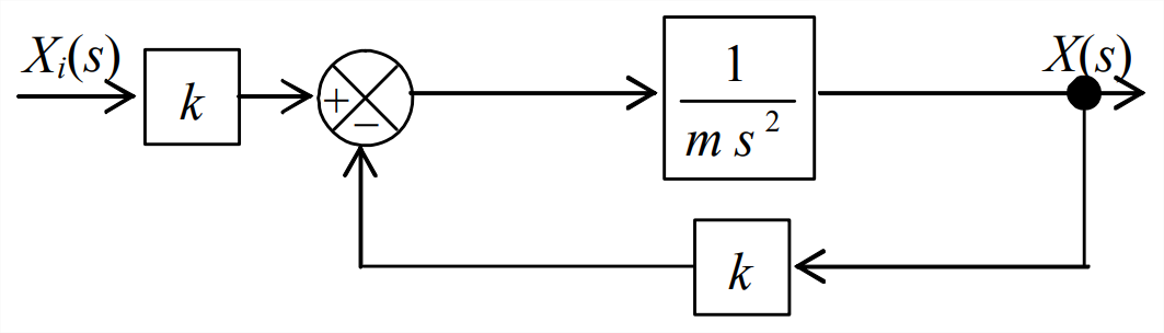
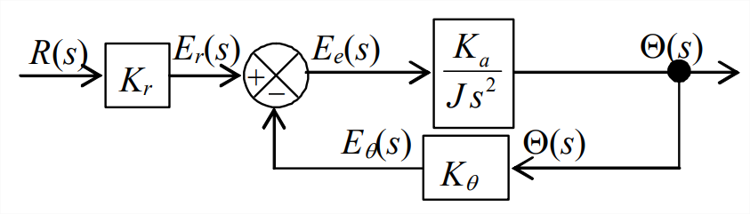
In order to describe the motivation for this new feature of the control design, let us revisit the base-excited \(m\)-\(c\)-\(k\) system of Sections 13.2 and 13.3. The principal elements of Figure 13.2.3, that system’s Laplace block diagram, are reproduced on Figure \(\PageIndex{2}\). The inner feedback loop makes Figure \(\PageIndex{2}\) more complicated than any control system block diagram that we have encountered previously in this chapter. Consider, however, the case of zero damping, \(c = 0\), for which the system is an undamped, base-excited mass-spring (\(m\)-\(k\)) system, and Figure \(\PageIndex{2}\) loses the inner feedback loop, taking on the simpler appearance of Figure \(\PageIndex{3}\). Now, let us compare the Laplace block diagram of the base-excited (\(m\)-\(k\)) system with that of the rotor position-feedback control system, Figure \(\PageIndex{4}\), which is repeated here. The Laplace block diagrams of the two systems have nearly identical forms, with, for example, constants \(K_r\) and \(K_{a} / J\) in Figure \(\PageIndex{4}\) being directly analogous, respectively, to constants \(k\) and \(1 / m\) in Figure \(\PageIndex{3}\). Only the possibility on Figure \(\PageIndex{4}\) that input block constant \(K_{r}\) and feedback block constant \(K_{\theta}\) can be different keeps Figure \(\PageIndex{4}\) from being completely analogous to Figure \(\PageIndex{3}\). This is a minor difference that has no substantive effect in the following discussion.
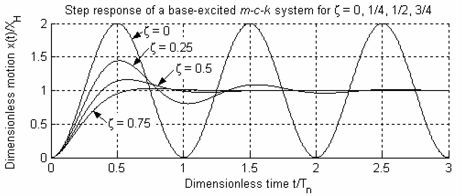
Let us exploit the similarities between the base-excited \(m\)-\(c\)-\(k\) system and the rotor-position control system in order to guide us toward a method for improving the latter. First, we refer back to the solution in Section 13.3 for response of the base-excited \(m\)-\(c\)-\(k\) system to step input \(x_{i}(t)=X_{H} H(t)\). The step response is presented graphically on Figure \(\PageIndex{5}\), which is repeated on the next page for your convenience.
Recall the following definitions for the \(m\)-\(c\)-\(k\) system: \(\omega_{n}=\sqrt{k / m}\), \(T_{n}=2 \pi / \omega_{n}\), and \(\zeta=c /(2 \sqrt{m k})\). Note on Figure \(\PageIndex{5}\) that the addition of positive damping (\(c>0 \Rightarrow \zeta>0\)) to the undamped system produces output \(x(t)\) that approximates the input; therefore, the positively damped \(m\)-\(c\)-\(k\) system is, indeed, a suitable control system, whereas the undamped \(m\)-\(k\) system is not.
Can we modify the undamped rotor-position control system in such a way that it has the same type of positive damping, and therefore suitable control performance, as the \(m\)-\(c\)-\(k\) system? Block diagram Figure \(\PageIndex{2}\) for the positively damped \(m\)-\(c\)-\(k\) system suggests that we might improve the rotor-position control system by adding an inner feedback loop to its block diagram, Figure \(\PageIndex{4}\), a loop that is similar to the inner loop of Figure \(\PageIndex{2}\). But are there practical physical operations and devices corresponding to the purely mathematical addition of this type of loop to Laplace block diagram Figure \(\PageIndex{4}\)? To answer this question, let us observe that the Laplace feedback signal of the inner loop on Figure \(\PageIndex{2}\) is \(s X(s)\), which is the Laplace transform of velocity \(\dot{x}(t)\). Therefore, the inner loop on Figure \(\PageIndex{2}\) represents mathematically the physical operations of detecting the output velocity and multiplying that velocity by negative constant \(−c\) to create a damping force that opposes motion of mass \(m\). We can perform the analogous physical operation for the rotor-position control system by measuring output rotational velocity \(p(t) \equiv \dot{\theta}(t)\) with an appropriate sensor (such as a rate gyroscope) and feeding that signal negatively back to the input of the actuator. Figure \(\PageIndex{6}\) depicts the modified rotor-position control system, with both this rate feedback (to provide positive damping) and the original position feedback (to provide positive stiffness).
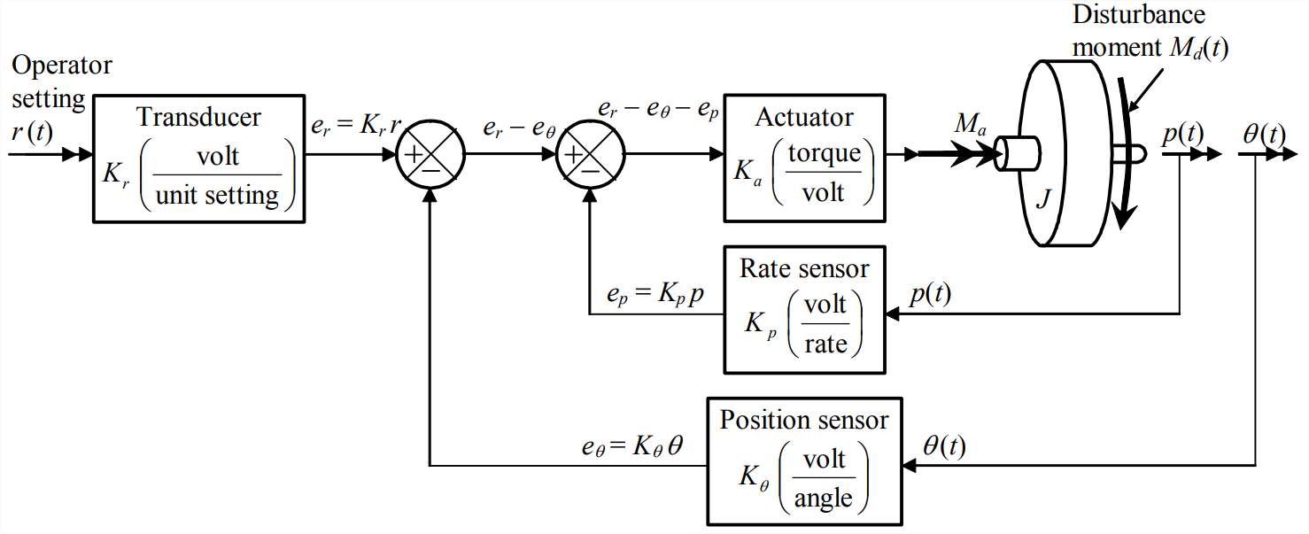
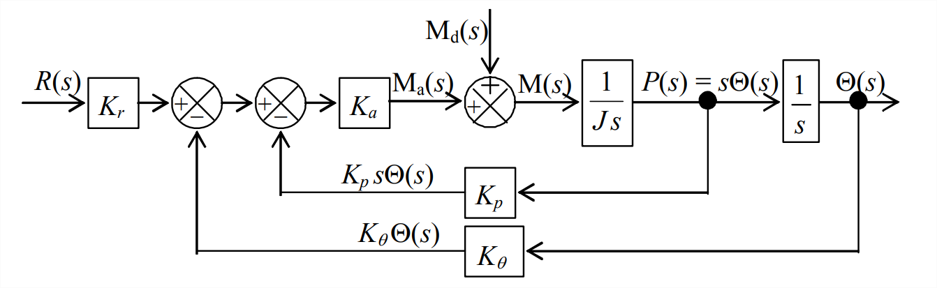
Figure \(\PageIndex{7}\) is the Laplace block diagram corresponding to functional diagram Figure \(\PageIndex{6}\). For measuring and feeding back the rotational velocity, the appropriate form of plant ODE of motion Equation 14.1.1 is \(J \dot{p}=M(t)\), so the appropriate plant transfer function in the new inner loop is \(L[p(t)] / L[M(t)] \equiv P(s) / \mathrm{M}(s)=1 /(J s)\). Also, the definition of rotational velocity leads to the forward-branch integration transfer function, \(\Theta(s) / P(s)=1 / s\). Comparing Figure \(\PageIndex{7}\) with Figure \(\PageIndex{2}\) for the base-excited \(m\)-\(c\)-\(k\) system, we see that the two Laplace block diagrams have nearly identical forms, except for the presence of the disturbance moment on Figure \(\PageIndex{7}\). Thus, and to summarize, we have modified the rotor-position control system to add positive damping, using the base-excited \(m\)-\(c\)-\(k\) system as a model.
The position-feedback and rate-feedback types of control illustrated by Figures \(\PageIndex{6}\) and \(\PageIndex{7}\) are relatively simple output operations: this control involves no more than basic arithmetic operations on the sensed output signals, without any modification of the error signal in the forward branch. Chapter 15 introduces control by input error operations, which involves more general mathematical operations upon a single error signal.
Next, let us analyze in detail the SISO version of the modified rotor-position control system. Thus, we set \(M_{d}(t)=0\) and \(\mathrm{M}_{\mathrm{d}}(s)=0\), and we re-draw Figure \(\PageIndex{7}\) as SISO block diagram Figure \(\PageIndex{8}\). Our objectives are: first, to derive from Figure \(\PageIndex{8}\) the closed-loop transfer function, \(\operatorname{CLTF}(s) \equiv \Theta(s) / R(s)\); second, to infer from \(\operatorname{CLTF}(s)\) the characteristics of the SISO system.
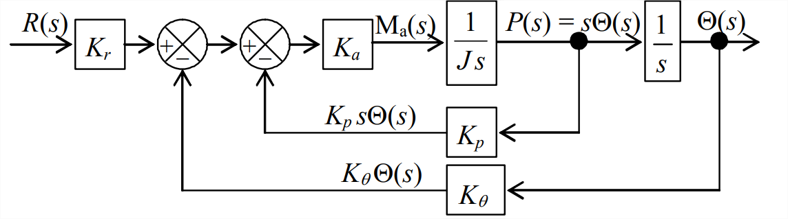
We could resolve block diagram Figure \(\PageIndex{8}\) by the “brute-force” method of applying Equation 14.4.7 first to the inner loop, then to the outer loop. However, we can achieve the same result more simply by using some sensible block-diagram algebra. The approach in each step is to modify a block and/or branch so as to simplify the diagram without changing the most important output signals. The obvious first step, is to combine the two blocks in the forward branch of the inner loop on Figure \(\PageIndex{8}\) into transfer function \(K_{a} /(J s)\).
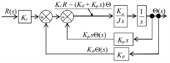
Next, we move the branch point of the inner loop to the right of the integration block, and modify accordingly the feedback transfer function of the inner loop, as shown below.
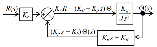
Next, we multiply the two blocks of the forward branch inside the loops into transfer function \(K_{a} /\left(J s^{2}\right)\). Now, both feedback branches essentially originate at the same branch point and terminate at the same summing junction, so we combine them into a single feedback branch with an appropriate transfer function, as shown at right. This block diagram has only a single loop, so we can apply Equation 14.4.7 with the following transfer-function polynomials: \(N_{G}=K_{a}\), \(D_{G}=J s^{2}\), \(N_{H}=K_{p} s+K_{\theta}\), and \(D_{H}=1\). The result is:
\[\frac{N_{G} D_{H}}{D_{G} D_{H}+N_{G} N_{H}}=\frac{K_{a} \times 1}{J s^{2} \times 1+K_{a} \times\left(K_{p} s+K_{\theta}\right)}=\frac{K_{a}}{J s^{2}+K_{a} K_{p} s+K_{a} K_{\theta}} \nonumber \]
Finally, multiplying this loop transfer function by the input transducer sensitivity gives
\[\operatorname{CLTF}(s) \equiv \frac{\Theta(s)}{R(s)}=\frac{K_{r} K_{a}}{J s^{2}+K_{a} K_{p} s+K_{a} K_{\theta}}\label{eqn:14.20} \]
Let us cast system transfer function Equation \(\ref{eqn:14.20}\) into a form that displays more clearly the fundamental characteristics of the closed-loop system. We again use as a guide the base-excited \(m\)-\(c\)-\(k\) system of Section 13.2. The undamped natural frequency of that system is \(\omega_{n}=\sqrt{k / m}\), and the viscous damping ratio is \(\zeta=c /(2 \sqrt{m k})\). Using these definitions, we can express transfer function Equation 13.2.3 in terms of these fundamental system characteristics rather than the physical parameters \(m\), \(c\), and \(k\):
\[T F(s) \equiv \frac{X(s)}{X_{i}(s)}=\frac{k}{m s^{2}+c s+k}=\frac{k / m}{s^{2}+(c / m) s+k / m}=\frac{\omega_{n}^{2}}{s^{2}+2 \zeta \omega_{n} s+\omega_{n}^{2}}\label{eqn:14.21} \]
Manipulating Equation \(\ref{eqn:14.20}\) in a similar manner, with an additional step to account for the possibility that \(K_{r} \neq K_{\theta}\), gives:
\[\operatorname{CLTF}(s) \equiv \frac{\Theta(s)}{R(s)}=\frac{K_{r}}{K_{\theta}} \times \frac{K_{a} K_{\theta} / J}{s^{2}+\left(K_{a} K_{p} / J\right) s+K_{a} K_{\theta} / J}=\frac{K_{r}}{K_{\theta}} \times \frac{\omega_{n}^{2}}{s^{2}+2 \zeta \omega_{n} s+\omega_{n}^{2}}\label{eqn:14.22} \]
In Equation \(\ref{eqn:14.22}\) the undamped natural frequency and viscous damping ratio of the rotor-position control system are
\[\omega_{n}=\sqrt{\frac{K_{a} K_{\theta}}{J}} \quad \text { and } \quad \zeta=\frac{K_{a} K_{p}}{2 J \omega_{n}}\label{eqn:14.23} \]
Equation \(\ref{eqn:14.22}\) differs in form from Equation \(\ref{eqn:14.21}\) only in the presence of pseudo-static multiplier \(K_{r} / K_{\theta}\), which is defined in Equation 14.3.5.
The system with transfer function Equation \(\ref{eqn:14.21}\) behaves as a control system should: in this case, as a positively damped, 2nd order system. For example, if the parameters in Equation \(\ref{eqn:14.22}\) are selected such that \(\zeta\) is in the range 0.3 to 0.5, and if the operator setting is step function \(r(t)=R_{H} H(t)\), then the inverse Laplace transform developed in homework Problem 9.12 gives the type of step response shown on the figure at right. The output cannot exactly follow this infinitely fast input, but it rises quickly and settles quickly to the desired pseudo-static response. This example illustrates a general characteristic of control systems: it is generally impossible to achieve absolute accuracy instantly (in this case, the pseudo-static response), but a good control system can achieve practically acceptable accuracy, with a practically acceptable time lag between the input and the desired output.
It was observed earlier that position feedback through the sensor with gain \(K_{\theta}\) has the effect of attaching between the operator setting and the rotor inertia an artificial restoring spring with stiffness constant \(K_{a} K_{\theta}\). We see now, additionally, that rate feedback through the sensor with gain \(K_{p}\) has the effect of imposing upon the absolute motion of the rotor an artificial viscous damper with damping constant \(K_{a} K_{p}\).
Finally, let us note that the favorable and stable performance of this rotor-position control system is strongly dependent upon the positivity of constants \(K_{a} K_{\theta}\) and \(K_{a} K_{p}\). In practice, it is possible (in fact, too easy) to make these constants negative, usually by accident or negligence, which could cause the system to be unstable. Chapters 16 and 17 examine in more detail the important issue of system stability.