14.7: Chapter 14 Homework

1. In Section 14.3 for the rotor-position control system with position feedback, the transfer function relating output rotor position to input operator setting, with zero disturbance, is derived by a series of block-diagram algebraic operations to resolve (simplify) Figure 14.3.3. In practice, for assessment of control system quality, it is often required also to determine the transfer function that relates output rotor position to the disturbance, with zero operator setting. The appropriate block diagram for that task in this case comes from Figure 14.3.2, with \(R(s) = 0\), as shown at left. Derive from this block diagram the transfer function \(\frac{\Theta(s)}{\mathrm{M}_{\mathrm{d}}(s)}=\frac{1}{J s^{2}+K_{e} K_{\theta}}\). This task is not difficult: just write \(\mathrm{M}_{\mathrm{a}}(s)\) in terms of \(\Theta(s)\), then \(\mathrm{M}(s)=\mathrm{M}_{\mathrm{a}}(s)+\mathrm{M}_{\mathrm{d}}(s)\), and \(\mathrm{M}(s) \times 1 / J s^{2}=\Theta(s)\), which steps should lead you to the required result. This result can also be derived directly from the ODE of motion Equation 14.3.4, but the assignment here is to derive it from the block diagram, to give you practice with block-diagram algebra.

   

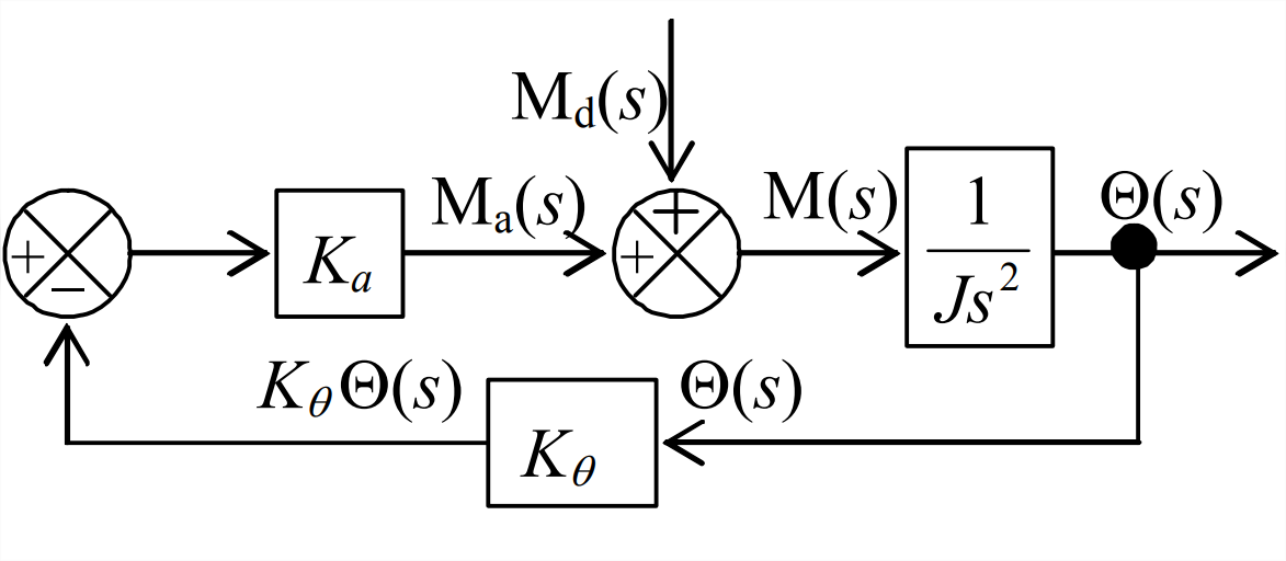
   Figure \(\PageIndex{1}\) (Copyright; author via source)

2. In some systems, information is fed forward as well as backward. Each of the Laplace block diagrams Figure \(\PageIndex{2}\) and \(\PageIndex{3}\) shown below includes both a feedforward branch and a unity-feedback branch. Transfer functions \(F(s)\) and \(G(s)\) represent arbitrary plant, filter, sensor, etc. system elements. (We could also include a transfer-function block in the unity-feedback branch, but its value would be simply 1, so it is standard practice to omit that obvious block.) For the part(s) assigned, derive the algebraic equation for the system transfer function, \(X(s) / R(s)\), in terms of \(F(s)\) and \(G(s)\).

   1. 

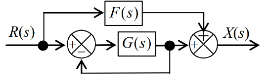
      Figure \(\PageIndex{2}\) (Copyright; author via source)

   2. 

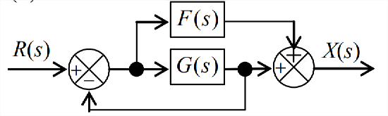
      Figure \(\PageIndex{3}\) (Copyright; author via source)

   3. The idealized series damper-spring high-pass mechanical filter shown in Figure 3.7.4 has the governing ODE with right-hand-side (RHS) dynamics, \(\dot{x}_{o}+\left(1 / \tau_{1}\right) x_{o}=\dot{x}_{i}(t)\), Equation 3.7.6. The transfer function from this ODE is clearly \(X_{o}(s) / X_{i}(s)=s /\left(s+1 / \tau_{1}\right)\), where \(L\left[x_{i}(t)\right] \equiv X_{i}(s)\) and \(L\left[x_{o}(t)\right] \equiv X_{o}(s)\). With the definition of a new independent variable \(x_{d}(t)\) and the auxiliary equation \(x_{o}(t)=x_{d}(t)+x_{i}(t)\), the ODE is converted into an alternate form without RHS dynamics, \(\dot{x}_{d}+\left(1 / \tau_{1}\right) x_{d}=-\left(1 / \tau_{1}\right) x_{i}(t)\), Equation 3.7.8. Construct a Laplace block diagram using the alternate ODE and the auxiliary equation; this diagram should have input \(X_{i}(s)\) on the left and output \(X_{o}(s)\) on the right, and it should include a feedforward branch. Use block-diagram algebra on this diagram to derive again the system transfer function \(X_{o}(s) / X_{i}(s)=s /\left(s+1 / \tau_{1}\right)\).
3. Consider a system represented by the somewhat general Laplace block diagram at the right. Constant \(K_{r}\) is an input sensor gain, and transfer functions \(G_{1}(s)\), \(G_{2}(s)\), \(H_{1}(s)\), and \(H_{2}(s)\) represent arbitrary plant, filter, sensor, etc. system elements. Use block-diagram algebra to show in detail that the closed-loop transfer function is \[\operatorname{CLTF}(s) \equiv \frac{X(s)}{R(s)}=\frac{K_{r} G_{1} G_{2}}{1+G_{1} H_{1}+G_{1} G_{2} H_{2}} \nonumber \]

   

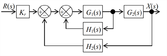
   Figure \(\PageIndex{4}\) (Copyright; author via source)

4. Consider a system represented by the block diagram below. The feedback branch is a unity-feedback path; we could include a transfer-function block in that branch, but its value would be simply 1, so it is standard practice to omit that obvious block.
   1. Show that the closed-loop transfer function is\[C L T F(s)=\frac{X(s)}{R(s)}=\frac{10(s+1)}{s^{2}+10 s+10} \nonumber \]

      

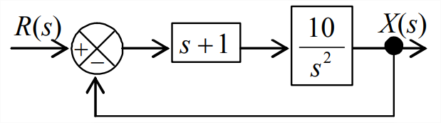
      Figure \(\PageIndex{5}\) (Copyright; author via source)

   2. Evaluate the denominator quadratic equation to calculate the viscous damping ratio \(\zeta\), which should indicate that the closed-loop system is overdamped.
   3. Factor the denominator quadratic into the form \(\left(s-p_{1}\right)\left(s-p_{2}\right)\), find the values of poles \(p_{1}\) and \(p_{2}\). (partial answer: \(p_{1}=-1.127\) s⁻¹)
   4. Suppose that the ICs are zero and that the input is a step function, \(r(t)=5 H(t)\). Determine the complete algebraic equation for output \(x(t)\). First express \(X(s)\) in a partial-fraction expansion, then find the inverse Laplace transform. Use your \(x(t)\) equation to find the final value, \(\lim _{t \rightarrow \infty} x(t)\), after all dynamic motion has damped out. (partial answer: one of the terms in the equation for \(x(t)\) should be \(-5.728 e^{-8.873 t}\).)
5. Consider position control of a reaction wheel (from Section 3.3) by position feedback plus rate feedback, for which the system Laplace block diagram is:

   

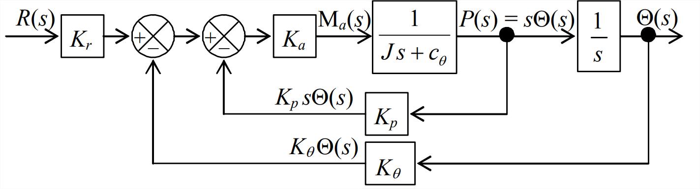
   Figure \(\PageIndex{6}\) (Copyright; author via source)

   This block diagram is identical to Figure 14.5.8, except that the plant transfer function from Equation 3.3.2 is \(1 /\left(J s+c_{\theta}\right)\), not just \(1 / J s\), due to the presence of bearing friction with assumed viscous damping constant \(c_{\theta}\). The following data were measured for a small laboratory reaction-wheel assembly:\[J=2.56 \times 10^{-3} \mathrm{lb} \text { -inch-sec }^{2}, c_{\theta}=0.020 \frac{\text { ounce inch }}{\mathrm{rad} / \mathrm{s}}, K_{a}=0.950 \frac{\text { ounce inch }}{\mathrm{V}} \nonumber \]For the case(s) assigned, the control system transducer and sensor sensitivities are as shown in columns 2, 3, and 4 of the following table:

   Case	\(K_{r}\) (V/rad)	\(K_{\theta}\) (V/rad)	\(K_{p}\) (Vs/rad)	\(t_{r}\) (s)	\(\bar{x}_{p}\)
   1	15	10	0.36	0.1280	0.3858
   2	1.5	1.5	0.27	0.4507	0.1117
   3	14	21	0.35	0.08163	0.5355
   4	3.5	3.5	0.24	0.2255	0.3260

   1. Calculate from the values in table columns 2, 3, and 4 the following quantities for this closed-loop system: pseudo-static multiplier \(K_{r} / K_{\theta}\), undamped natural frequency \(\omega_{n}\) (rad/s), viscous damping ratio \(\zeta\), and damped natural frequency \(\omega_{d}\) (rad/s).
   2. Suppose that the input is a step function, \(r(t)=R_{H} H(t)\), with magnitude \(R_{H}=30\) degrees. For the subsequent step response, calculate the rise time \(t_{r}\), the peak time \(t_{p}\), the maximum overshoot ratio \(\bar{x}_{p}\), and the settling time \(t_{s}\) (see Section 9.8). Also, calculate the final static value of wheel position, \(\lim _{t \rightarrow \infty} \theta(t)\) in degrees, after all dynamic motion has damped out. Partial answers are given in columns 5 and 6 of the table above to help you know if you are, or are not on the right track, but you still must show all derivations and calculations leading to these answers.
   3. For the same step input as in part 14.5.2, use MATLAB to calculate and plot the step response \(\theta(t)\) in degrees from \(t=0\) until at least the settling time \(t=t_{s}\).
6. In Section 14.5 for the rotor-position control system with position feedback and rate feedback, the transfer function relating output rotor position \(\Theta(s)\) to input operator setting \(R(s)\), with zero disturbance, is derived by a series of block-diagram algebraic operations to resolve (simplify) Figure 14.5.8. In practice, for assessment of control system quality, it is often required also to determine the transfer function that relates output rotor position to the disturbance, with zero operator setting. The appropriate Laplace block diagram for that task in this case comes from Figure 14.5.7, with \(R(s) = 0\), as shown on the figure at right. Derive from this block diagram the algebraic equation for transfer function \(\frac{\Theta(s)}{\mathrm{M}_{\mathrm{d}}(s)}\).

   

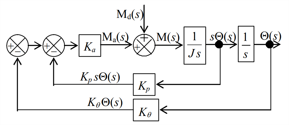
   Figure \(\PageIndex{7}\) (Copyright; author via source)

7. Consider a system represented by the Laplace block diagram at right. The outer feedback branch is a unity feedback path; we could include a transfer-function block in that branch, but its value would be simply 1, so it is standard practice to omit that obvious block.

   

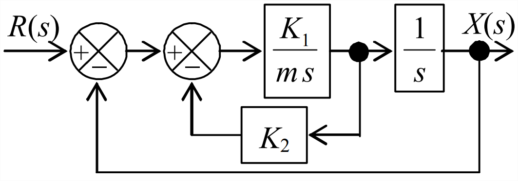
   Figure \(\PageIndex{8}\) (Copyright; author via source)

   1. Use the result of Problem 14.3 or any other method of your choice to show that the closed-loop transfer function is \[\frac{X(s)}{R(s)}=\frac{K_{1}}{m s^{2}+K_{1} K_{2} s+K_{1}} \nonumber \]
   2. Suppose that the ICs are zero and that the input to this system is a step function, \(r(t) = R_{H} H(t)\). For the case(s) assigned, the value of the mass-like parameter \(m\) (in consistent units) is given in column 2 of the table below. Calculate the values of constants \(K_1\) and \(K_2\) (in consistent units) that will produce the values of maximum overshoot ratio \(\bar{x}_{p}\) and peak time given in columns 3 and 4 of the table (see Section 9.8). Note that this is a design exercise: you are calculating values of system parameters that are intended to produce specified control objectives. Complete the problem by calculating also the rise time \(t_r\) and the settling time \(t_s\). Partial answers are given in columns 5 and 6 of the table below to help you know if you are, or are not on the right track, but you still must show all derivations and calculations leading to these answers.
   3. Let the step magnitude of part 14.7.2 be \(R_{H}=0.753\) (in consistent units). Calculate the final value, \(\lim _{t \rightarrow \infty} x(t)\), after all dynamic motion has damped out.