15.5: Chapter 15 Homework

1. Consider closed-loop transfer function Equation 15.4.3, with definitions Equation 15.4.4, for position control of a rotor by an ideal PD controller.
   1. Suppose that we know rotational inertia \(J\), actuator sensitivity \(K_{a}\), and equal input and feedback transducer sensitivities, \(K_{r}=K_{\theta}\), and that we want to specify (i.e., “design”) the undamped natural frequency \(\omega_{n}\) and the viscous damping ratio \(\zeta\) for this controlled system. Hence, we need to determine appropriate values for proportional gain \(P\) and derivative time constant \(\tau_{d}\), which we would set in the PD controller. For a particular system, we have \(J=2.56 \mathrm{e}-3\) lb-s²-inch (the value for a small aluminum wheel about four inches in diameter, Figure 3.3.1), and the product \(K_{r} K_{a}=0.0350\) lb-inch/rad; let us specify \(f_{n}=\omega_{n} / 2 \pi=1.00\) Hz (so that step-response rise time will be around ¼ s) and \(\zeta=+0.1\) (too low for most practical control systems, but it suits the overall purposes of this problem). Calculate the required values of \(P\) and \(\tau_{d}\) (s).
   2. Use the MATLAB residue operation (see homework Problem 2.15) to expand the transfer function [with the numerical values of part 15.1.1] into a partial-fraction expansion. The poles are critical to the stability of any system, which is the subject of Chapter 16. For this system, you should find a pair of poles that are complex conjugates, and their real part should be negative—this means that the system is stable.
   3. Let the input be a step, \(r(t)=R_{H} H(t)\). First, apply the final-value theorem to find \(\lim _{t \rightarrow \infty} \theta(t)\). Next, use inverse transforms Equations 15.2.22 and 15.2.23 [or just appropriately adapt step response Equation 15.2.24 to this case] to show that the step response is \[\theta(t)=R_{H}\left[1-e^{-\zeta \omega_{n} t}\left(\cos \omega_{d} t-\frac{\zeta \omega_{n}}{\omega_{d}} \sin \omega_{d} t\right)\right], \text { for }|\zeta|<1 \text { and } \omega_{d}=\omega_{n} \sqrt{1-\zeta^{2}} \nonumber \]Finally, let the input step magnitude be \(R_{H}=0.1\) radian, with the numerical values of part 15.1.1, and use MATLAB to plot the output \(\theta(t)\) over the time interval 0-2.5 s, about 2½ cycles.
   4. To simulate what would happen if you made a mistake and got the wrong sign for \(\tau_{d}\) (and therefore for \(\zeta\)), let \(\zeta=-0.1\), and repeat the operations of parts 15.1.2 and 15.1.3. If you can plot \(\theta(t)\) for both \(\zeta=+0.1\) and \(\zeta=-0.1\) on the same graph, it will enhance comparison of the two cases. For \(\zeta=-0.1\), you should find the real part of the complex conjugate poles to be positive; the associated time history \(\theta(t)\) should indicate system instability. Observe for this unstable system that the final-value theorem incorrectly predicts a finite steady-state value for this step response.
2. Consider ideal PID control of the position of a rotor that has significant inertia \(J\). Let us also account for a disturbance moment \(M_{d}(t)\) acting upon the rotor. The Laplace block diagram for this 3^rd order system is drawn above. In the following exercises, assume that this system is stable.

   

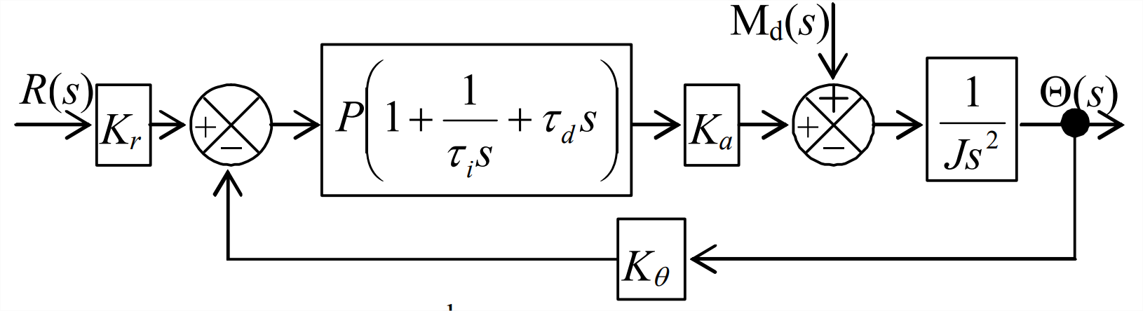
   Figure \(\PageIndex{1}\) (Copyright; author via source)

   1. For zero disturbance, \(\mathrm{M}_{\mathrm{d}}(s)=0\), derive the algebraic equation for closed-loop transfer function\(\Theta(s) / R(s)\). For step input, \(r(t)=R_{H} H(t)\), apply the final-value theorem to find \(\lim _{t \rightarrow \infty} \theta(t)\).
   2. For zero input, \(R(s)=0\), derive the algebraic equation for closed-loop transfer function \(\Theta(s) / \mathrm{M}_{\mathrm{d}}(s)\). For step disturbance, \(M_{d}(t)=M_{H} H(t)\), apply the final-value theorem to find \(\lim _{t \rightarrow \infty} \theta(t)\). A control system should suppress permanent output due to a step disturbance.
3. Consider PI control of the speed (not position) of a rotor that has significant inertia \(J\). The sensor on the output is a tachometer with gain constant \(K_p\), so the electrical signal that is fed back is \(K_{p} \dot{\theta}\). (This configuration illustrates a general rule-of-thumb in control-system design: sense and feed back the quantity that you want to control.) This is a simplified model, for example, of an automobile’s cruise-control system. Let us also allow for a disturbance moment \(M_{d}(t)\) acting upon the rotor. The Laplace block diagram for this system is at left.

   

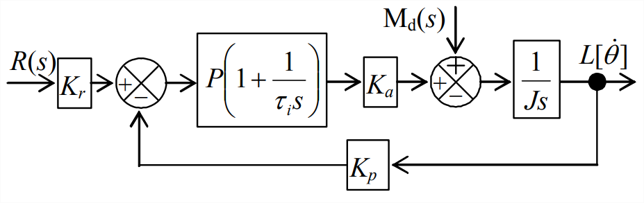
   Figure \(\PageIndex{2}\) (Copyright; author via source)

   1. For zero disturbance, \(\mathrm{M}_{\mathrm{d}}(s)=0\), derive the algebraic equation in terms of all parameters on the Laplace block diagram for the closed-loop transfer function \(L[\dot{\theta}] / R(s)\) that relates output rotational velocity \(\dot{\theta}(t)\) to input command \(r(t)\). For step input, \(r(t)=R_{H} \times H(t)\), apply the final-value theorem to find the algebraic equation for \(\lim _{t \rightarrow \infty} \dot{\theta}(t)\), assuming that this asymptotic value exists. Explain (perhaps using an example from your own experience, such as a cruise-control system) the physical significance of the ratio \(K_{r} / K_{p}\) of the input-transducer sensitivity to the tachometer sensitivity.
   2. Derive algebraic equations for undamped natural frequency \(\omega_{n}\) and viscous damping ratio \(\zeta\) of this controlled system, in terms of inertia \(J\), actuator sensitivity \(K_{a}\), tachometer sensitivity \(K_{p}\), proportional gain \(P\), and integral time constant \(\tau_{i}\).
4. In this problem, you will produce graphically and compare the frequency-response functions of the exact, but physically unrealizable differentiator \(x_{d} \equiv \dot{e}_{e}\) (which is used in this book for ideal PD control) and an approximate, but physically realizable differentiator that has the character of a high-pass filter.
   1. Section 15.4 gives the ODE of the approximate differentiator as \(\varepsilon \tau_{d} \dot{x}_{d}+x_{d}=\dot{e}_{e}\), with \(\tau_{d}\) being the positive derivative time constant and \(\mathcal{E}\) being a small positive number in the range 0.1-0.3; show that the complex frequency-response function (FRF) of output signal \(x_{d}(t)\) relative to input signal \(e_{e}(t)\) is \(F R F(\omega)=j \omega /\left(1+j \omega \varepsilon \tau_{d}\right)\).
   2. For frequency response, the input signal has the steady-state sinusoidal form \(e_{e}(t)=E_{e} \cos \omega t\) and the output signal has the corresponding form \(x_{d}(t)=X_{d}(\omega) \cos (\omega t+\phi)\). Use the FRF of part 15.4.1 to show that the equations for FRF magnitude ratio and phase of the approximate differentiator are \(\frac{X_{d}(\omega)}{\omega_{b} E_{e}}=\frac{\bar{\omega}}{\sqrt{1+\bar{\omega}^{2}}}\) and \(\phi(\omega)=\frac{\pi}{2}-\tan ^{-1} \bar{\omega}\), in which the break frequency is \(\omega_{b} \equiv 1 /\left(\varepsilon \tau_{d}\right)=2 \pi f_{b}\) and the dimensionless frequency ratio is \(\bar{\omega} \equiv \omega / \omega_{b}=f / f_{b}\). Use the magnitude-ratio equation to derive equations for the low-frequency and high-frequency asymptotes, and sketch those asymptotes on a log-log graph such as Figure 4.3.3. The approximate differentiator should exhibit the character of a high-pass filter, analogous to the system of homework Problem 4.4. Use the asymptotes as an envelope to guide you in sketching the actual curve of \(X_{d}(\omega) /\left(\omega_{b} E_{e}\right)\), as is done on Figure 4.3.3. Finally, on a semi-log graph below the log-log graph (analogous to Figure 4.3.2), sketch the variation with frequency of phase \(\phi(\omega)\).
   3. Now consider the exact differentiator, with equation \(x_{d} \equiv \dot{e}_{e}\). Repeat all the steps of parts 15.4.1 and 15.4.2 for the exact differentiator, sketching the magnitude-ratio and phase curves on the part 15.4.2 graphs, but in some different color or line style, so that the curves for exact and approximate differentiators are clearly distinguishable. You should be able to infer from these final graphs the ranges of frequency over which the approximate differentiator is reasonably accurate, or inaccurate.
5. Consider the transfer function of the PD-controlled rotor position of Section 15.4, Equation 15.4.3 with equal input and feedback transducer sensitivities, \(K_{r}=K_{\theta}\), in the form \(\frac{\Theta(s)}{R(s)}=\frac{K_{r} P K_{a}\left(1+\tau_{d} s\right)}{J s^{2}+K_{r} P K_{a} \tau_{d} s+K_{r} P K_{a}}\). Use this transfer function and the block diagram of Figure 15.4.2 to write the algebraic equation for the transfer function of the PD controller, \(W(s) / R(s)\). Now, examine the nature of \(W(s) / R(s)\) in the following steps:
   1. Find the order \(m\) of the numerator polynomial and the order \(n\) of denominator polynomial of \(W(s) / R(s)\). Is this transfer function causal or acausal, and what does that mean in theory regarding the physical realism of \(W(s) / R(s)\)?
   2. Suppose that the input is the infinitely fast step function \(r(t)=R_{H} H(t)\) of homework Problem 15.1.3. Show that the controller-output transform \(W(s)\) must have a constant direct term, as defined in homework Problem 2.15. What is the component of time response \(w(t)\) that corresponds to the direct term of \(W(s)\), and is this a physically realizable signal from a real device? Your conclusions from parts 15.5.1 and 15.5.2 should be compatible.
   3. If you conclude in parts 15.5.1 and 15.5.2 that something is physically unrealistic about these theoretical results, then what is there in the theoretical analysis that makes the results defective? Propose a remedy that should produce physically realizable results, and show succinctly, with appropriate algebraic equations and written explanation (but no calculations), why your proposed remedy should work.
6. Consider control of a spacecraft’s pitch attitude, \(\theta(t)\), for which the ODE of motion, from Equation 14.2.4, is J \ddot{\theta}=M_{a}(t)+M_{d}(t), where \(M_{d}(t)\) is a disturbance moment. In this problem, you will apply a physically realizable form of PD control, with the control actuator moment defined as \(M_{a}(t)=K_{a} \times w(t)\), where \(K_{a}\) is the actuator sensitivity. The output signal from the realizable PD controller is \(*w(t)=P\left[e_{e}(t)+\tau_{d} x_{d}(t)\right]\), where \(x_{d}(t)\) is the dependent variable in the ODE \(\varepsilon \tau_{d} \dot{x}_{d}+x_{d}=\dot{e}_{e}\) (see the relevant discussion in Section 15.4). The input error is \(e_{e}(t)=K_{r} r(t)-K_{\theta} \theta(t)\), where \(r(t)\) is the input operator setting, and \(K_r\) and \(K_\theta\) are the transducer sensitivities at, respectively, the input and output feedback.
   1. Draw and label completely the Laplace block diagram of this system, from input \(R(s)\equiv L[r(t)]\) to output \(\Theta(s) \equiv L[\theta(t)]\), including disturbance moment signal \(\mathrm{M}_{\mathrm{d}}(s)=L\left[M_{d}(t)\right]\).
   2. For \(\mathrm{M}_{\mathrm{d}}(s)=0\), derive from the block diagram of part 15.6.1 the closed-loop transfer function \(\operatorname{CLTF}(s)=\Theta(s) / R(s)=\operatorname{Num}(s) / \operatorname{Den}(s)\), where \(\operatorname{Num}(s)\) and \(\operatorname{Den}(s)\) are polynomials in powers of \(s\). Partial answer: \(\operatorname{Den}(s)=J s^{2}\left(\varepsilon \tau_{d} s+1\right)+P K_{a} K_{\theta}\left[\tau_{d}(1+\varepsilon) s+1\right]\)
   3. For step input, \(r(t)=R_{H} H(t)\), apply the final-value theorem to find \(\lim _{t \rightarrow \infty} \theta(t)\), provided that the system is stable.
   4. How does \(\operatorname{CLTF}(s)\) in part 15.6.2, for a physically realizable form of PD control, differ from the corresponding closed-loop transfer function that applies for an ideal but unrealizable PD controller, for which \(w(t)=P\left[e_{e}(t)+\tau_{d} \dot{e}_{d}(t)\right]\)? [Do not re-derive this \(\operatorname{CLTF}(s)\) from scratch; instead, just make a simple substitution in the \(\operatorname{CLTF}(s)\) of part 15.6.2.] Discuss in one or two sentences.
7. Consider the “position actuator” depicted on functional diagram Figure 15.2.2, which represents a system for control of a rotor immersed in a viscous liquid. Suppose that the position actuator is the rotor-position control system of Figure 14.5.6, and that Figure 14.5.7 is the actuator’s Laplace block diagram. Your assignment in this problem is to revise the immersed-rotor control system’s Laplace block diagram, Figure 15.2.3, to incorporate the position-actuator dynamics, replacing the simplified block of actuator gain \(K_{a}\) with an appropriate version of Figure 14.5.7, and making any other necessary modifications. There are at least three significant changes required, the first two being notational. (1) You should re-label the input of the modified Figure 14.5.7 to \(W(s) \equiv L[w(t)]\), replacing \(R(s)\), and also re-label the output to \(\Theta_{a}(s) \equiv L\left[\theta_{a}(t)\right]\), replacing \(\Theta(s)\). (2) In order to avoid notational ambiguity, you should re-label all system components on Figure 14.5.7 having subscripted symbol \(K\), with subscripted symbol \(Q\), e.g., on the revised Figure 14.5.7, \(K_{r} \rightarrow Q\), and \(K_{a} \rightarrow Q\), etc. (3) It is necessary to recognize that the rotational spring with stiffness \(k_{\theta}\) shown on Figure 15.2.2 imposes upon the position actuator a moment \(k_{d}\left(\theta-\theta_{a}\right)\). The quantities labeled on Figures 14.5.6 and 14.5.7 that can represent moment \(k_{d}\left(\theta-\theta_{a}\right)\) are, respectively, \(M_{d}(t)\) and \(\mathrm{M}_{\mathrm{d}}(s)\), for example, \(\mathrm{M}_{\mathrm{d}}(s)=k_{\theta}\left[\Theta(s)-\Theta_{a}(s)\right]\). (However, the moment \(k_{\theta}\left(\theta-\theta_{a}\right)\) is clearly defined and not at all random or unpredictable mathematically, so it is not truly a disturbance in the sense defined in Section 14.2, with reference to Figure 14.2.1.) Accounting for items (1)-(3) and any other necessities, draw a Laplace block diagram of the immersed-rotor control system, a diagram that incorporates the position-actuator dynamics from Figure 14.5.7. This block diagram will be somewhat longer than others appearing in this book. It is not required that you simplify this block diagram to derive an algebraic expression for the closed-loop transfer function; it is possible to do so using the operations of block-diagram algebra described in Chapters 13 and 14, but the process would be complicated algebraically, and it would produce a very long and messy equation for \(\operatorname{CLTF}(s)\). Modern processes using specialized computer software are more appropriate than algebra-by-hand for a task such as this. For example, if you had numerical values for all the system parameters (\(J\), \(k_{\theta}\), \(Q_{r}\), \(\dots\), \(\tau_{1}\), \(P\), etc.), then you could easily generate a single equation for \(\operatorname{CLTF}(s)\) with MATLAB by using the functions tf, and feedback, and series (or, rather than series, simply the operation of transfer function multiplication).